U.S. Open Data — Gathering and Understanding the Data from 2018 Shinnecock

After losing in a playoff to make it out of the local qualifying for the 2018 US Open at Shinnecock, I’m stuck at my apartment watching everyone struggle, wondering how much I’d be struggling if I was there myself.

Besides on TV, the US Open website offers some other way to follow what players are doing. As shown here, they very generously give us information on everyone’s shots on different holes. We’re able to see where people hit the ball, on which shot, and what their resulting score was on the hole. For example, why in the world did Tony Finau, the currently second ranked longest hitter on tour, hit it short off the first tee, leave himself 230 yards to the hole where he makes bogey?

Why didn’t Tony rip D?

One of the cool things these images show is the groupings of all the shots on a hole, like the tee shots here. And when I see very specific and interactive data like we have here, I know it comes from somewhere that I’m able to see myself. So I figured I should grab that data and do some cluster analysis on different holes to see if there are certain spots that players like to hit it.

Here, I’ll go through the data we have, what the values and the numbers mean, and also the code I wrote to eat up the data and display the graphs. Once I have this part going, I’ll be able to perform further analysis to most things that come to mind.

Any questions, comments, concerns, trash talking, get in touch: twitter, contact.

Current Posts

Using Clustering Algorithms to Analyze Golf Shots

Finding the data

First step was to search for where the data for the hole insights page was coming from. As always, open the dev tools, click on the network tab, and find what’s getting called with a pretty name.

Alert!

The file itself is quite dense and has all the information, which is really cool! It has IDs for all the players, all the shots they have on the hole, which include the starting distance from the flag and the ending distance to the flag.

First off, we’re given a list of Ps, meaning an array of player information, like this:

...
{u'FN': u'Justin', u'ID': u'33448', u'IsA': False, u'LN': u'Thomas', u'Nat': u'USA', u'SN': u'THOMAS'},
{u'FN': u'Dustin', u'ID': u'30925', u'IsA': False, u'LN': u'Johnson', u'Nat': u'USA',u'SN': u'JOHNSON D'}
{u'FN': u'Tiger', u'ID': u'08793', u'IsA': False, u'LN': u'Woods', u'Nat': u'USA', u'SN': u'WOODS'}
...

It looks like we have first name, player’s ID, whether or not they’re an amateur, last name, nationality, scoreboard name. The important part of this information is the ID, where we’ll be able to match players to shots.

Next, we’re given a few stats on the hole for the day:

Continue reading

Predicting PGA Tour Scoring Average from Statistics Using Linear Regression

First off, I admit, that’s probably the most boring title for a blog post ever. It gets a negative value on the clickbait scale that is generally unseen in the modern, “every click equals dollars” era that we live in. On the other hand, it tells you exactly what this article is about — predicting scoring average using stats.

In this article, I’ll go through getting the data from the database, cleaning that data for use, and then running a linear regression in order to generate coefficients for each of the stats to generate scoring average predictions. Oh, and some analysis and commentary at the end!

Shameless shoutout to my other blog, Golf on the Mind. Check it out and subscribe to the newsletter / twitter / instagram if you’re into golf at all. Or ignore, and keep reading for some code!

Here's a pic of a golf course to get you in the mood.

Here’s a pic of a golf course to get you in the mood.

Getting the data

Last time if you remember, I spent all this effort taking the csv stat files, and putting the information into a database. Start there if you haven’t read that post yet. It’ll show how I grabbed the stats and formatted them.

Now that you’re back in the present we need to create a query that gets the stats for the players for a specific year. An example row in a CSV file of the data would be something like:

player_id, player_name, stat_1_value, stat_2_value, … , stat_n_value

for stats 1 to n where n (the number of stats), and the which stats themselves (driving distance, greens in regulation, etc.) vary depending on inputs.

Now let me say, I am not an expert in writing sql queries. And since people on the internet loooove to dole out hate in comments sections, I’m just going to say that there’s probably a better way of writing this query. Feel free to let me know and I can throw an edit in here, but this query works just fine.

select players.id,
  players.name,
  max(case when stat_lines.stat_id=330 then stat_lines.raw else null end) as putting_average,
  max(case when stat_lines.stat_id=157 then stat_lines.raw else null end) as driving_distance,
  max(case when stat_lines.stat_id=250 then stat_lines.raw else null end) as gir,
  max(case when stat_lines.stat_id=156 then stat_lines.raw else null end) as driving_accuracy,
  max(case when stat_lines.stat_id=382 then stat_lines.raw else null end) as scoring_average
from players
  join stat_lines on stat_lines.player_id = players.id
  join stats on stat_lines.stat_id=stats.id
where stat_lines.year=2012 and (stats.id=157 or stats.id=330 or stats.id=382 or stats.id=250 or stats.id=156) and stat_lines.raw is not null
group by players.name,players.id;

High level overview time! We’re selecting player id, and player name, along with their stats for putting average, driving distance, greens in regulation, driving accuracy and scoring average for the year 2012. In order to get the right stats, we need to know the stat id for the stats.

One more thing. This query is funky, and I probably could have designed the schema differently to make this prettier. For example, I could have just gone with one table, stat_lines, with fields for player_name and stat_name (along with all the current fields) and then the sql would be very simple. But there are other applications to keep in mind. What if you wanted to display all stats by a player? Or all of a players stats for a certain year? With the way I have the schema set up, those queries are simple and logical. For this specific case, I’ll deal with the complexity.

Loading the Data

That query above is great, but it’s not going to cut it if I have to specify what the year, and the stat ids in that string every time I run the script. Gotta be dynamic here.

Continue reading

Python, Postgres, SQLAlchemy, and PGA Tour Stats

A little ago, I wrote an article about scraping a bunch of PGA Tour stats. The end result of that was writing those stats out into CSV files. While this was suitable for that task of gathering the stats, let’s face it, you’re probably going to want to put those into some database to allow for easier querying, or possibly integrate it into to web app in the future. There are a bunch of different reasons for wanting this, so I’m going to go through the process I took to put all the data in the CSV files into the database.

Adding players to the database

First step is to fire up postgres! I’m not going to cover starting postgres since there’s so much good content about it, for example, this super good tutorial here by Digital Ocean. I created at database called ‘pgatour’, created a user named ‘pgatour_user’ with password ‘pgatour_user_password’, logged in, and created the first table, Player.

pgatour=# create table players (
  id serial PRIMARY KEY,
  name varchar (255) NOT NULL
);

Ok, now, as a test, I’m going to add myself into the database from the psql command line.

pgatour=# insert into players (name) values ('Jack Schultz')

Note that since id is serial, we don’t need to insert that value, just the name. Alas, I am not on the PGA Tour, so I’m going to need to delete myself.

pgatour=# select * from players;
id | name
----+--------------
1 | Jack Schultz
(1 row)

pgatour=# delete from players where name = 'Jack Schultz';
DELETE 1
pgatour=# select * from players;
id | name
----+------
(0 rows)

Looking good. Now onto the Python side.

Python SQL Alchemy Interface

Now that the Players table in the database is set up, we’re going to want to be able to modify the contents of it in Python.

Continue reading

Gather all the PGA Tour stats

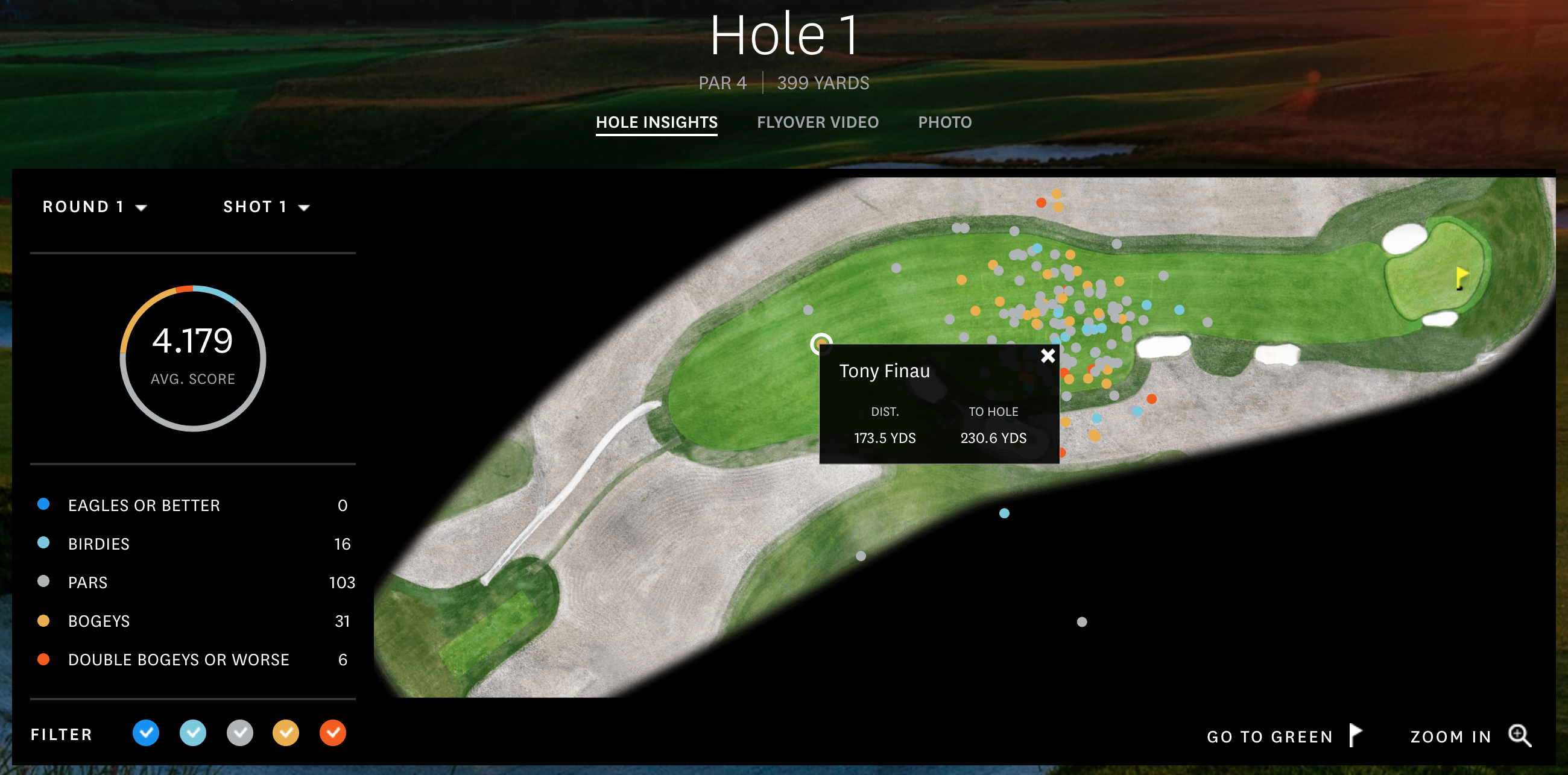
As someone who likes writing and investigating data sets, and as a huge fan of golf (and writer of a golf blog, Golf on the Mind), when I realized that the PGA Tour website has a crap ton of stats about players on the PGA Tour going back to the early 80s, I figured there was definitely some investigating to do. And the first step, as with any data analysis, is getting the data into a standard and usable form. And in reality, you’ll find this effort takes up most of your time if you do this sort of thing.

So before I can start looking at anything interesting, I need to do some scraping. This article will take you through that process.

UPDATE — 5/25/18 — I get way too many questions about whether the data is available, so I went back through and updated the code and currently scraping it every week. I’m not going to post the link here, but shoot me an email and I can go ahead and share the links.

Step 1 — Downloading the HTML files

The usual process for scraping, is to grab the html page, extract the data from that page, store that data. Repeat for however many web pages have the data you want. In this case however I wanted to do something different. Instead of grabbing the data from a web page and storing that data, I wanted to actually store the html file itself as a first step. Only after would I deal with getting the info from that page.

Reasoning behind this was to avoid unnecessarily hitting pgatour.com’s servers. Undoubtedly, when scraping, you’ll run into errors in your code – either missing data, oddly formatted data you didn’t account for, or any other random errors that can happen. When this happens, and you have to go back and grab the web page again, you’re both wasting time by grabbing the same file over the internet, and using up resources on that server’s end. Neither a good result.

So in my case here, I wrote code to download and save the html once, and then I can extract data as I please from those files without going over the internet. Now for the specifics.

On pgatour.com, the stats base page is located at pgatour.com/stats.html. If you notice at the top. This will land you at the overview page, but you can notice at the top there are eight categories of stats: Off the Tee, Approach the Green, Around the Green, Putting, Scoring, Streaks, Money/Finishes, and Points/Rankings. Under each of these categories are a list of stats in a table. Clicking on any of those links and you’ll get the current year’s stats for all the qualifying players. On the side, you’ll notice a dropdown where you can select the year you want the stat for. Our goal is to get the pages for each of those stats, for every year offered, and save the page in a directory named for the stat, and the year as the filename.

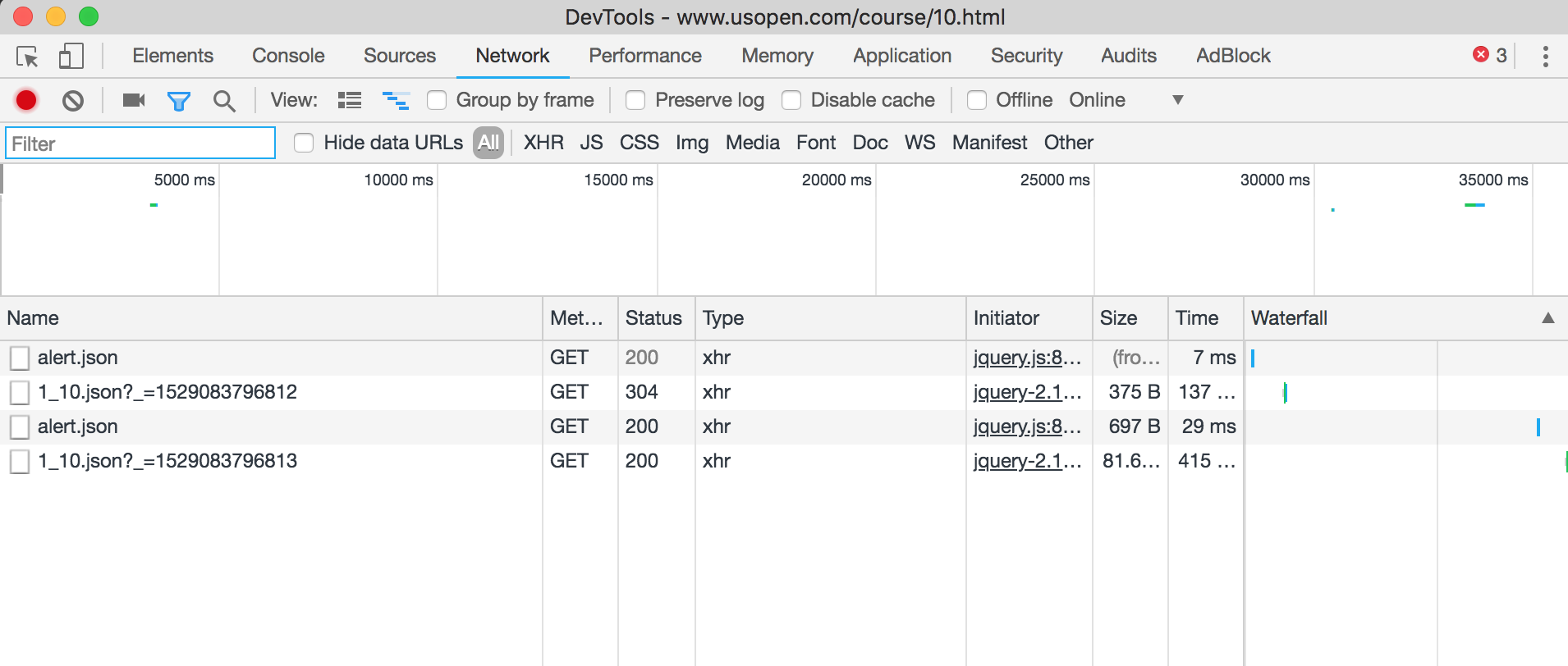
The url pattern when you’re on a single stat is straight forward. For example the url for current Driving Distance is http://www.pgatour.com/stats/stat.101.html, and the url for Driving Distance in 2015 is http://www.pgatour.com/stats/stat.101.2015.html. Simply injecting the year into the url after the stat id will get you what you need.

In order to get the different stats from the category page, we’re going to loop the categories, yank out url and name for a stat, grab the current page, see which years the stat is offered for, generate the required urls, and loop those urls saving the page! Reading the code should make this make more sense.

The last issue with grabbing the html pages is how long it takes. In the end, we’re talking about over 100 stats, with about 15-20 years of history. At first, I wanted to play nice not overwhelm the pgatour.com servers, but then I realized that pgatour.com can probably handle the load since they need to be able to deal with the constant refreshing that people do when checking leaderboards at the end of a tournament. Thankfully, python’s Gevent library allows us to easily, in parallel, grab pages and save them. After all that explanation, take a look at the code I used to save the files.

url_stub = "http://www.pgatour.com/stats/stat.%s.%s.html" #stat id, year
category_url_stub = 'http://www.pgatour.com/stats/categories.%s.html'
category_labels = ['RPTS_INQ', 'ROTT_INQ', 'RAPP_INQ', 'RARG_INQ', 'RPUT_INQ', 'RSCR_INQ', 'RSTR_INQ', 'RMNY_INQ']
pga_tour_base_url = "http://www.pgatour.com"
def gather_pages(url, filename):
 print filename
 urllib.urlretrieve(url, filename)

def gather_html():
 stat_ids = []
 for category in category_labels:
 category_url = category_url_stub % (category)
 page = requests.get(category_url)
 html = BeautifulSoup(page.text.replace('\n',''), 'html.parser')
 for table in html.find_all("div", class_="table-content"):
   for link in table.find_all("a"):
     stat_ids.append(link['href'].split('.')[1])
 starting_year = 2015 #page in order to see which years we have info for
 for stat_id in stat_ids:
   url = url_stub % (stat_id, starting_year)
   page = requests.get(url)
   html = BeautifulSoup(page.text.replace('\n',''), 'html.parser')
   stat = html.find("div", class_="parsys mainParsys").find('h3').text
   print stat
   directory = "stats_html/%s" % stat.replace('/', ' ') #need to replace to avoid
   if not os.path.exists(directory):
     os.makedirs(directory)
   years = []
   for option in html.find("select", class_="statistics-details-select").find_all("option"):
     year = option['value']
     if year not in years:
       years.append(year)
   url_filenames = []
   for year in years:
     url = url_stub % (stat_id, year)
     filename = "%s/%s.html" % (directory, year)
     if not os.path.isfile(filename): #this check saves time if you've already downloaded the page
       url_filenames.append((url, filename))
     jobs = [gevent.spawn(gather_pages, pair[0], pair[1]) for pair in url_filenames]
     gevent.joinall(jobs)

Step 2 — Convert HTML to CSV

Now that I have the html files for every stat, I want to go through the process of getting the info from the tables in the html, into a consumable csv format. Luckily, the html is very nicely formatted so I can actually use the info. I saved all the html files in a directory called stats_html, and I basically want to create the same folder structure in a top level directory I’m calling stats_csv.

Steps in this task are 1) Read in the files, 2) using Beautiful Soup, extract the headers for the table, and then all of the data rows and 3) write that info as a csv file. I’ll just go right to the code since that’s easiest to understand as well.


for folder in os.listdir("stats_html"):
 path = "stats_html/%s" % folder
 if os.path.isdir(path):
   for file in os.listdir(path):
   if file[0] == '.':
     continue #.DS_Store issues
   csv_lines = []
   file_path = path + "/" + file
   csv_dir = "stats_csv/" + folder
   if not os.path.exists(csv_dir):
     os.makedirs(csv_dir)
   csv_file_path = csv_dir + "/" + file.split('.')[0] + '.csv'
   print csv_file_path
   if os.path.isfile(csv_file_path): #pass if already done the conversion
     continue
   with open(file_path, 'r') as ff:
     f = ff.read()
     html = BeautifulSoup(f.replace('\n',''), 'html.parser')
     table = html.find('table', class_='table-styled')
     headings = [t.text for t in table.find('thead').find_all('th')]
     csv_lines.append(headings)
     for tr in table.find('tbody').find_all('tr'):
       info = [td.text.replace(u'\xa0', u' ').strip() for td in tr.find_all('td')]
     csv_lines.append(info)
     #write the array to csv
     with open(csv_file_path, 'wb') as csvfile:
       writer = spamwriter = csv.writer(csvfile, delimiter=',')
       for row in csv_lines:
         writer.writerow(row)

And that’s it for the scraping! There are still a couple issues before you can actually use the data, but those issues are dependent on what you’re trying to find out. The big example being getting the important piece of info from the csv. Some of the stats are percentage based stats, others are distance measured in yards. There are also stats measured in feet / inches (23’3″ for example). Also an issue is that sometimes, the desired stat is in a different column in the csv file depending on the year the stat is from. But like I said, those issues aren’t for an article on data scraping, but we’ll have to deal with them when looking at the data later.

Weekly Fantasy Golf Results and a System of Linear Equations

I had an idea recently about how to use the “wisdom of the crowds” in forecasting performance for weekly fantasy golf. I see the benefits of crowdsourcing all the time working with prediction markets at Inkling Markets, so I figured I could leverage that to get an edge when choosing my lineups. I’ll get into the details of how I’m doing that in a later post since that’s worthy on it’s own, but I found a subproblem that I’d have to solve in order to make it work.

While some of the sites offer player salaries in an easily digestible csv format, they’re a little stingy when it comes to results. They only keep contest results for the last 30 days, and the only downloadable results they offer are the results from contests in the past week, which just show point totals for an entire lineup, not the point totals for individual golfers. And I need those player’s points for testing my forecasting algorithm, as well as using them in making the actual forecasts. One way to figure this out is to scrape the hole by hole data from pgatour.com and apply the site’s scoring algorithm to each of those holes, but I’ve found a better, simpler, and much more elegant solution.

I can model the results csv file as a system of linear equations, and by converting the different user’s lineups into a matrix and vector those equations, numpy can solve for the point totals that each golfer earned during the tournament.

Here’s an example row from that file, with the person’s username hidden.

"Rank","EntryId","EntryName","TimeRemaining","Points","Lineup"
263,85826104, "UNAME (1/100)", 0, 430.50, "(G) Ryan Palmer ,(G) Pat Perez ,(G) Kevin Kisner ,(G) Ben Martin ,(G) Shawn Stefani ,(G) John Peterson "

In order to solve, we need to create two data structures. The first is a num_lineups by num_players matrix of coefficients, where the value is a 1 if the player was used in that lineup, and 0 if he wasn’t. The second is an array of total points scored by that lineup.

The idea is that if we had an array of the points the players scored over the course of the tournament, we should be able to take the dot product of that and the corresponding row in the coefficient matrix to generate the point total of that lineup.

Here’s the code to generate the coefficient matrix and the point array:

points_label = "Points"
lineup_label = "Lineup"
player_coefficients = []
lineup_points = []
with open('outcome.csv', 'rb') as csvfile:
  rows = csv.reader(csvfile)
  headers = rows.next()
  points_index = headers.index(points_label)
  lineup_index = headers.index(lineup_label)
  for row in rows:
    points = float(row[points_index])
    lineup_points.append(points)
    names = [name.strip() for name in row[lineup_index].replace('(G)','').split(',')]
    lineup_players = [0] * player_count
    for name in names:
      lineup_players[player_list.index(name)] = 1
      player_coefficients.append(lineup_players)

From here, all we need to do is convert those arrays into numpy arrays, and run numpy’s linear algebra least squares algorithm to get the solution array!

coefficient_matrix = np.array(player_coefficients)
point_array = np.array(lineup_points).transpose()
solution = np.linalg.lstsq(coefficient_matrix, point_array)
player_points = list(solution[0])

Initially, I tried to use the numpy’s solve algorithm, but by looking at the docs realized that solve dealt with square coefficient matrices (something that I still remember from all those math classes). The lstsqrs method is used to get approximate results from rectangular matrices as is the case here.

Printing out the results yields the following results for the top and bottom 10:

Chris Kirk: 126.0
Jason Bohn: 105.5
Brandt Snedeker: 102.0
Jordan Spieth: 101.5
Kevin Kisner: 99.0
George McNeill: 96.5
Pat Perez: 95.0
Adam Hadwin: 92.0
Ian Poulter: 87.5
Brian Harman: 87.0
...
Kenny Perry: 18.0
Jason Kokrak: 17.5
Jonas Blixt: 16.5
Corey Pavin: 16.0
Bo Van Pelt: 15.0
David Toms: 14.0
Brian Davis: 11.5
Tom Watson: 4.61852778244e-13
Tom Purtzer: 3.87245790989e-13
Scott Stallings: 2.84217094304e-13

Chris Kirk won so him having the highest point total makes sense, and the three guys at the bottom with zero points all withdrew so they should be at 0 points. Unfortunate for the guys who didn’t take them out of their lineups, but they gotta pay a little more attention!

Only issue with the final result is that I only end up with point totals from 117 players, when 133 teed it up at the beginning of the tournament. That means that we’re missing point totals from some of the guys. That being said, I’m going to assume that those players weren’t picked because they weren’t likely to play well, so hopefully that 117 offer a good representation of point totals. Also, could easily be that draftkings in this case only listed 117 players to choose from. I’ll need to investigate this week.

In the end, it took about 3 hours to write the code and write this post. It’s fun little problems like this that really remind you that programming is fun and has value. Being able to create technical solution to something you’re interested in is probably the best part about being a programmer. Check out the entire script in this gist.

Follow on twitter.