First off, I admit, that’s probably the most boring title for a blog post ever. It gets a negative value on the clickbait scale that is generally unseen in the modern, “every click equals dollars” era that we live in. On the other hand, it tells you exactly what this article is about — predicting scoring average using stats.
In this article, I’ll go through getting the data from the database, cleaning that data for use, and then running a linear regression in order to generate coefficients for each of the stats to generate scoring average predictions. Oh, and some analysis and commentary at the end!
Shameless shoutout to my other blog, Golf on the Mind. Check it out and subscribe to the newsletter / twitter / instagram if you’re into golf at all. Or ignore, and keep reading for some code!

Here’s a pic of a golf course to get you in the mood.
Getting the data
Last time if you remember, I spent all this effort taking the csv stat files, and putting the information into a database. Start there if you haven’t read that post yet. It’ll show how I grabbed the stats and formatted them.
Now that you’re back in the present we need to create a query that gets the stats for the players for a specific year. An example row in a CSV file of the data would be something like:
player_id, player_name, stat_1_value, stat_2_value, … , stat_n_value
for stats 1 to n where n (the number of stats), and the which stats themselves (driving distance, greens in regulation, etc.) vary depending on inputs.
Now let me say, I am not an expert in writing sql queries. And since people on the internet loooove to dole out hate in comments sections, I’m just going to say that there’s probably a better way of writing this query. Feel free to let me know and I can throw an edit in here, but this query works just fine.
select players.id,
  players.name,
  max(case when stat_lines.stat_id=330 then stat_lines.raw else null end) as putting_average,
  max(case when stat_lines.stat_id=157 then stat_lines.raw else null end) as driving_distance,
  max(case when stat_lines.stat_id=250 then stat_lines.raw else null end) as gir,
  max(case when stat_lines.stat_id=156 then stat_lines.raw else null end) as driving_accuracy,
  max(case when stat_lines.stat_id=382 then stat_lines.raw else null end) as scoring_average
from players
  join stat_lines on stat_lines.player_id = players.id
  join stats on stat_lines.stat_id=stats.id
where stat_lines.year=2012 and (stats.id=157 or stats.id=330 or stats.id=382 or stats.id=250 or stats.id=156) and stat_lines.raw is not null
group by players.name,players.id;
High level overview time! We’re selecting player id, and player name, along with their stats for putting average, driving distance, greens in regulation, driving accuracy and scoring average for the year 2012. In order to get the right stats, we need to know the stat id for the stats.
One more thing. This query is funky, and I probably could have designed the schema differently to make this prettier. For example, I could have just gone with one table, stat_lines, with fields for player_name and stat_name (along with all the current fields) and then the sql would be very simple. But there are other applications to keep in mind. What if you wanted to display all stats by a player? Or all of a players stats for a certain year? With the way I have the schema set up, those queries are simple and logical. For this specific case, I’ll deal with the complexity.
Loading the Data
That query above is great, but it’s not going to cut it if I have to specify what the year, and the stat ids in that string every time I run the script. Gotta be dynamic here.
You might think it’s a little janky that we’re just using raw sql to grab data instead of using one of those nice ORM libraries. If you want to do that for an exercise, go for it, but I’m not messing around with that when I can do string manipulations that return correct values.
One more thing to note about raw sql. Be really careful if you’re passing in user supplied values to a database. That’s a sql injection folks. ‘Bout as basic hacking as you can get. In this case, since it’s just a local script it’s fine, but if I used this in a web app where users could supply stats they wanted to see, then I’d have to be careful. As always, a relevant XKCD.
On to the code! First step is figuring out the ids of the different stats in the database, then we generate the query using information generated from the first db query that grabbed stat ids. As always, the code is easier to understand than me trying to explain in english.
stat_names = set([
 'Driving Distance',
 'Carry Distance',
 'Putting Average',
 'Greens in Regulation Percentage',
 'Greens or Fringe in Regulation',
 'Driving Accuracy Percentage',
 'Proximity to Hole',
 'Birdie Average',
 'Scrambling',
 'Scoring Average'
 ])

select_clauses = []
where_clauses = []
for stat_info in stats_info:
  stat_id = stat_info[0]
  stat_name = stat_info[1].lower().replace(' ','_')
  select_string = ", max(case when stat_lines.stat_id=%s then stat_lines.raw else null end) as %s" % (stat_id, stat_name)
  where_string = "stats.id=%s " % (stat_id)
  select_clauses.append(select_string)
  where_clauses.append(where_string)

underscored_stat_names = [stat_name.lower().replace(' ','_') for stat_name in stat_names if stat_name != 'Scoring Average']

sql_text = 'select players.id, players.name'
for select_clause in select_clauses:
  sql_text += select_clause
sql_text += '''
from players
join stat_lines on stat_lines.player_id = players.id
join stats on stat_lines.stat_id=stats.id
where
stat_lines.year=%s
and (
'''
for index, where_clause in enumerate(where_clauses):
if index != 0:
sql_text += 'or '
sql_text += where_clause
sql_text += '''
)
and stat_lines.raw is not null
group by players.name, players.id;
'''
Cleaning the Data
Next step is making sure that the data pulled from the database is clean and workable when passed into the linear regression.
Here’s how this part of the code is going to work. After getting the data, we loop through each stat in the stat_names variable and if we’ve defined a cleaning function for it, we map that Pandas row to the function and get back workable data.
Why do we want to do this? Some of the stats grabbed from pgatour.com aren’t in the correct form for running a linear regression. The big example here are the stats that are measured in feet and inches — like Proximity to Hole which measures the average proximity to the hole the player is in regulation. That data comes in the form of 30’6″. We need to turn that into a single number.
The way I decided to do this was create functions for each of the stats that need cleaning, and then dynamically call that function if it exists. Example below.
underscored_stat_names = [stat_name.lower().replace(' ','_') for stat_name in stat_names if stat_name != 'Scoring Average']

putting_average_clean = lambda x: float(x) * 18

def proximity_to_hole_clean(val):
  distances = str(val).split("'")
  inches = int(distances[0]) * 12 + int(distances[1][1:-1])
  return inches

df = pd.read_sql_query(sql_text_train, engine)
df = df[df.scoring_average.notnull()]
for underscored_stat_name in underscored_stat_names:
  try:
    cleaning_function = getattr(current_module, underscored_stat_name+'_clean')
    df[underscored_stat_name] = df[underscored_stat_name].map(cleaning_function)
  except AttributeError:
    pass
For each of the independent variables, we check to see if we’ve defined a cleaning function, and then map that function to each piece of data. In this case, we need to change proximity to hole to a float, and then also change putting average, which is measured in putts per hole, to putts per round which is easier to interpret.
Just a note, we could have done other functions on the data like normalization around 0, or scaling, but then we’d lose information later.
Running Linear Regression
Python, as pretty much every modern programming language these days, has a library that will run linear regression for you, removing the need to reimplement code that people have been using for years. Sure, there’s benefit in knowing the underlying code, but writing it yourself more than once probably is overkill.
To do the prediction, I used the statsmodel library’s OLS implementation. After getting the data from the database, dealing with cleaning the data, the code for linear regression here is very nice and simple.
We convert the stats to floats, we add a constant to the data frame, extract out the dependent variable, scoring average, then print out the summary from the fit and scatter actual and predicted!
import statsmodels.api as sm

X_train = df[underscored_stat_names].astype(np.float)
X_train = sm.add_constant(X_train)
y = df['scoring_average'].astype(np.float)

res = sm.OLS(y,X_train).fit()
print res.summary()
import matplotlib.pyplot as plt

fig, ax = plt.subplots()
ax.scatter(y_actual, ypred)
plt.show()
It’s fun to just play around with changing the variables we use in training. For example, what does the scatter plot look like if we just use one stat? Two stats? Is there a minimum amount and type of stat to use to get a good fit? What counts as a good enough fit? All questions worth exploring.
Thoughts!
Now is the time of the article where I point out interesting results from playing with the code!
Complementary stats — When I use multiple stats like greens in regulation, and greens or fringe in regulation, they’re basically the same thing. Same with Driving distance and carry distance. For example, in one of the runs using both driving distance and carry distance, the coefficients were -0.0024 and -0.0156 respectively. When only using driving distance in a subsequent run, the coefficient was -0.0182 which is 0.0002 off from -0.0024 + -0.0156. Also, the R squared values for each of the runs was equal at 0.782. In this case, you only need one.
Sign of the coefficient – When running the regression, OLS spits out the coefficients. For some stats, like driving distance, the coefficient is negative. For some other stats, putts per round for example, the coefficient is positive. Because of the linear nature of the math, these coefficients have an actual meaning, opposed to some other machine learning models. For example, if the coefficient for driving distance is the -0.0182 from above, every extra yard that you hit the golf ball equates to 0.0182 strokes off of your scoring average! So if you hit it ~54.9 yards further, expect to shoot a stroke lower on average.
R squared value – Besides just looking at the scatter plot and looking to see if we have a decent fit, OLS comes with the R squared value, which describes how good of a fit we have. Check out the wikipedia article for more information. Besides just having an empirical measure of how good the fit is, we can use R squared as a proxy for how important a stat is in determining a player’s scoring average.
As an example, let’s see which stat is “more important”, greens in regulation (short game) or proximity to hole. Both stats measure how close a player is to the hole when they get to the green. With the whole cocktail of stats, and using both GIR and proximity to hole, we get an R squared value of 0.798. Removing just GIR, the R squared value drops to 0.782. Removing just Proximity to hole, we get an R squared value of 0.791. Does this make sense? Sure, there’s more information encoded in proximity to hole variable since GIR just measure whether or not you were on the green, and not actually how close to the hole you were. So if you could only choose one of these variables to model on, go with proximity to hole.
One more example I tried is to see what’s more important, driving distance or driving accuracy. Quick results are that R squared with driving distance is 0.779, and with driving accuracy it drops to 0.744. Which suggests that driving distance is more important to scoring average than driving accuracy.
Time for me to preach some golf strategy here. Feel free to skip here if you aren’t interested in hearing about golf strategy, or don’t like hearing the truth. With that last run, I have numerical proof that it doesn’t matter if you hit the fairway, it just matters how far you hit the ball. So whenever you’re deciding whether to play safe with a 3 wood or iron off the tee, just rip driver. Being closer to the hole is so much more important than being in the fairway. We saw that the other week at the US Open at Oakmont. The scoring average for the two drivable par 4s was half a shot lower if the player hit driver off the tee compared to an iron. Seriously, just hit drivers folks.
Train set is better than predictions — From the two images below, can you tell which one is from the training set, and which one is using a different year’s data?
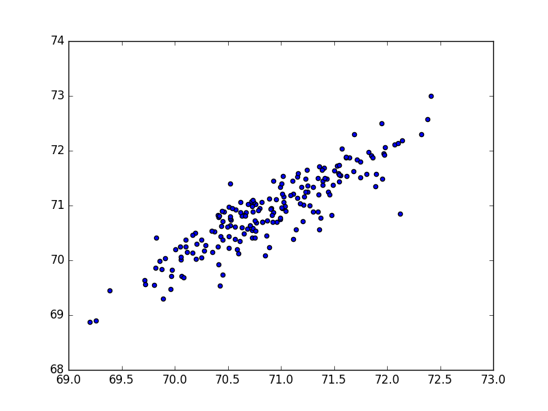
So pretty

Still pretty, but just not quite as pretty.
Yup, the top pic is predicting values on the training set, and the second is predicting values on a different data set. Still decent results, and you can see good correlation, but it isn’t as good. Just something to watch out for when you’re doing these machine learning projects. Everyone knows that what you train on and what you want to predict on is going to result in some loss of knowledge. but seeing it visually really hammers that idea home.
Possible non-linearity — Remember above when I said that 1 stroke less on average is equal to 54.9 yards? This easily might not be the case. Going from an average of 240 yards to 294.9 yards probably changes your scoring average more than going from 294.9 to 349.8 yards. In this data set, we’re only looking with professional golfers, so the range of driving distances goes from lowest of around 270 to the highest of around 310. The ranges for all the stats depend on the year, and also how depend on how the Tour measures the individual stats – whole other story with that. So within that range, the difference in advantage might approximate linearity, but it might be some other power.
For the Future
No post like this is complete without mentioning things I didn’t do, because let’s be honest, there’s always more interesting work to do with these types of questions.
Non-linear searching — As I mentioned in the non-linear section above, . We can achieve this by preprocessing the data by scaling it. Again though, we’re still dealing with human modification, and if we wanted really accurate results, it’d be better to use some model that automatically searches for scaled parameters.
Removing Putting Average — One thing to note, and what I didn’t expect to see, was that the coefficient for putting average wasn’t 1. Since we’re straight measuring measuring scoring average, we should be able to remove the 18 hole putting average from total average and run the regression again. Expectations are that coefficients would change.
Using ALL the Stats — If you look back at the scraping article, I ended up with a crap ton of random stats. Just a sample, I have over 30 different putting stats, all measuring how well a player putts. Clearly you don’t need that many for a simple model like linear regression here, but I would be curious to just throw all the different stats at this model and see how close we can approximate a player’s scoring average.

Pingback: What to Watch For in the 2017 Year of Golf | Golf On The Mind