Using Clustering Algorithms to Analyze Golf Shots from the U.S. Open

Cluster analysis can be considered one of the pillars of machine learning, and yet it’s one that’s difficult to talk about.

First off, it’s difficult to find specific use cases for clustering, other than pretty pictures. When looking through the wiki page on clustering, we’re told one of the uses is market research, where analysts use surveys to group together customers for market segmentation. That sounds great in theory, but the results don’t end with specific numbers telling the researchers what to do. Second, in so many cases, the hardest part of data science projects, or tutorials, is finding real world data that have the different results you want to show. In this case, I’m incredibly lucky.

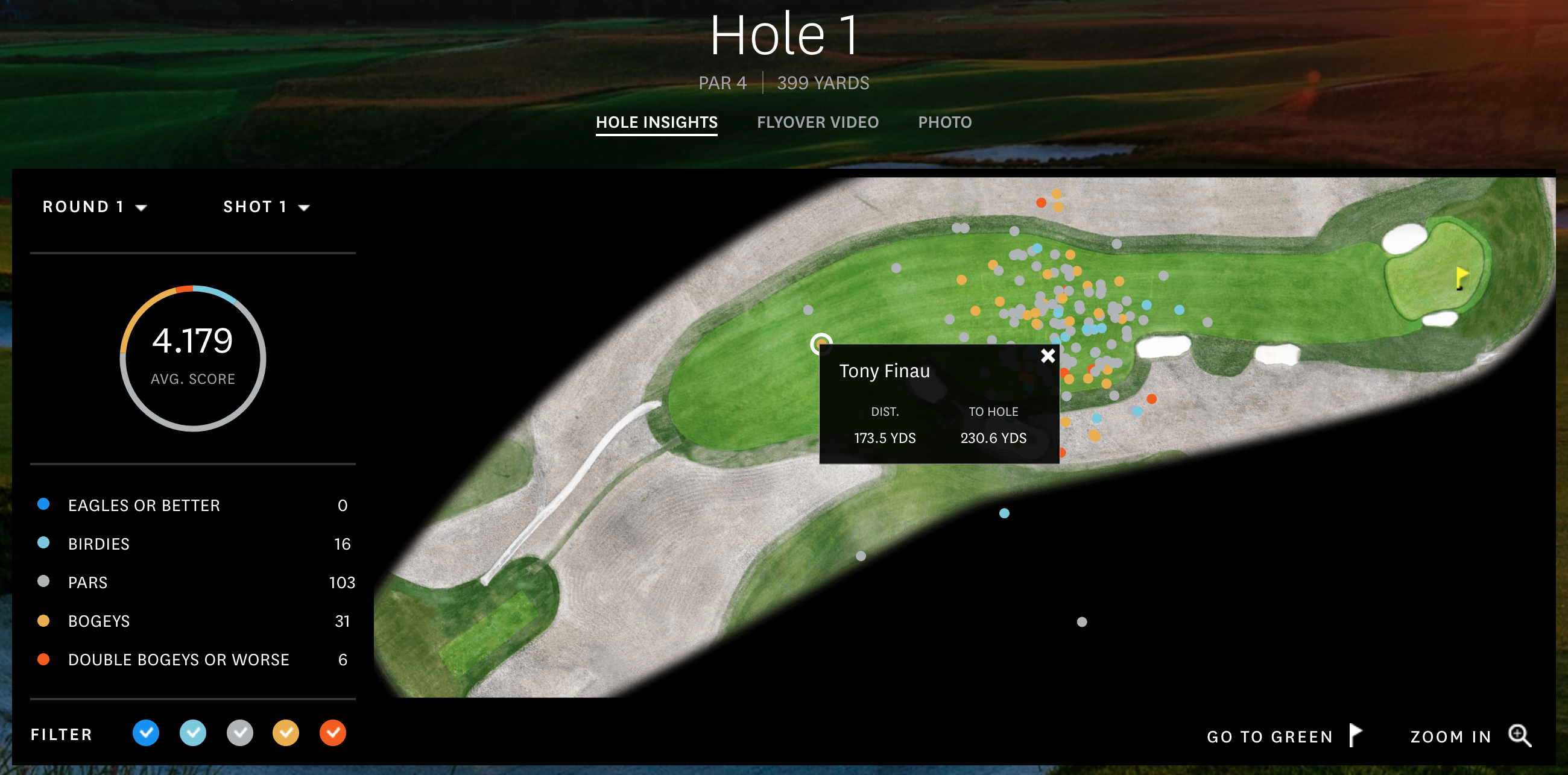
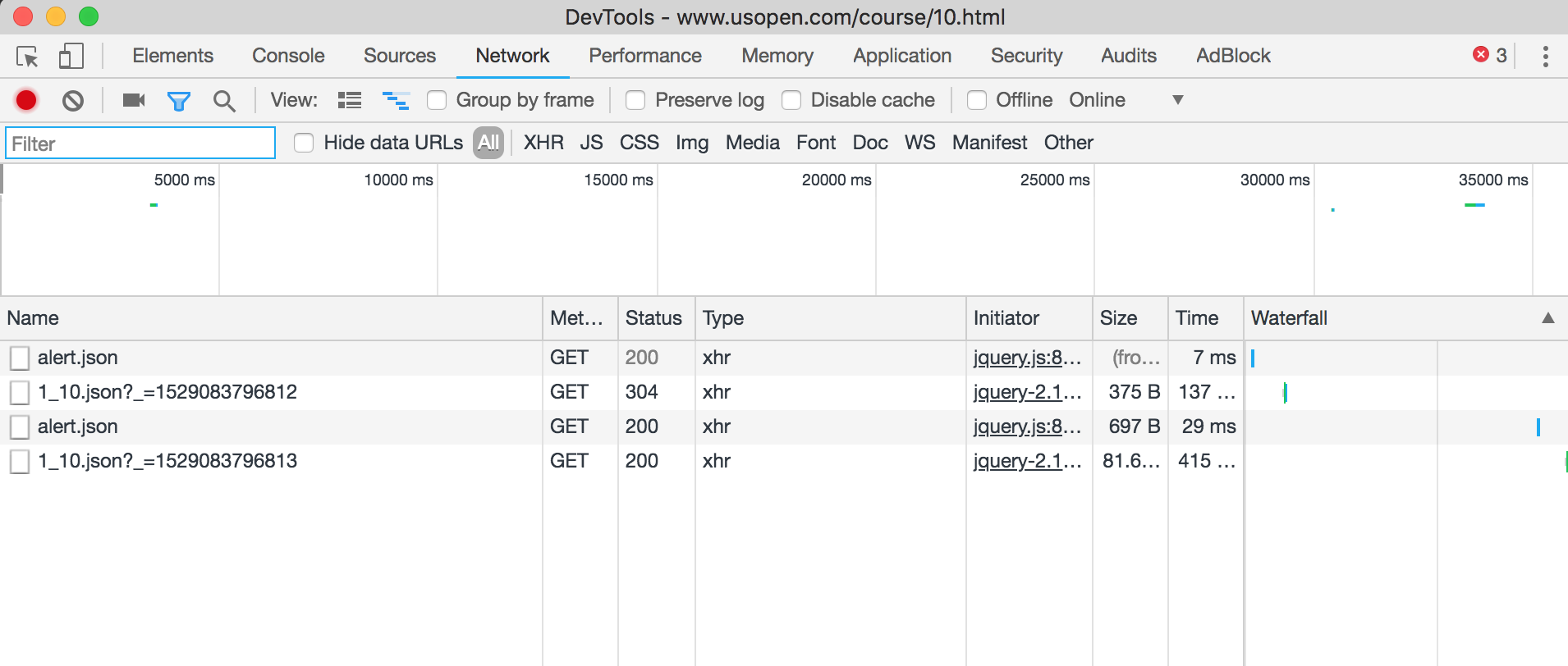
I have a golf background, and on U.S. Open’s website, they have these interactive graphs that show where each ball was located after each stroke for every player. If you click around, you can see who hit what shot, how far the shot went and how far remains between the ball and the hole. For cluster analysis, we’re going to use the location. For you to check out how I got the data, look and read here.

Shinnecock Hills, the host of the 2018 U.S. Open last week, has a few parts of the course where balls roll to collection areas into groups, or, ya know, clusters. Here are the specific shots our clustered data is coming from.

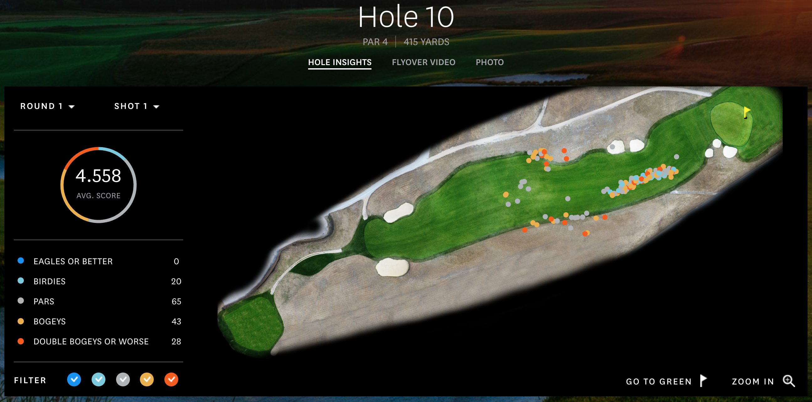
Hole 10, Round 1, Off the Tee

The description that the USGA gives hole number 10 is

The player faces a decision from the tee: hit a shot of about 220 yards to a plateau, leaving a relatively level lie, or drive it over the hill. Distance control is critical on the approach shot, whether from 180 yards or so to a green on a similar plateau, or with a shorter club at the bottom of the hill or, more dauntingly, part of the way down the hill. The approach is typically downwind, to a green with a closely mown area behind it.

First I’ll say, always hit driver off the tee. Look at the cluster! If you get it down the hill you’ll be in the fairway! In the vast, vast majority of the time, it’s better to be closer to the hole. Golf tips aside, when I first saw this graph, it popped out as a great example to use as a clustering example.

Shift command 4 if you want selective screenshots

When looking at this picture, the dots represent where the players hit their tee shots on hole 10 in the first round, and the colors show how many strokes it took them to finish the hole in relation to par. For this, we’re ignoring the final score and only looking at the shots themselves.

Hole 10, Round 1, Approaching the green

One data set isn’t good enough to demonstrate the differences of the algorithms, and I wanted to find an example of a green with collection areas that would make approach shots group together. Little did I know, the 10th green, the same hole as the one above showing the drives, is the best example out there. If you’re short, it rolls back to you. If you’re long, it rolls away. You gotta be sure to hit the green. You can see that here.

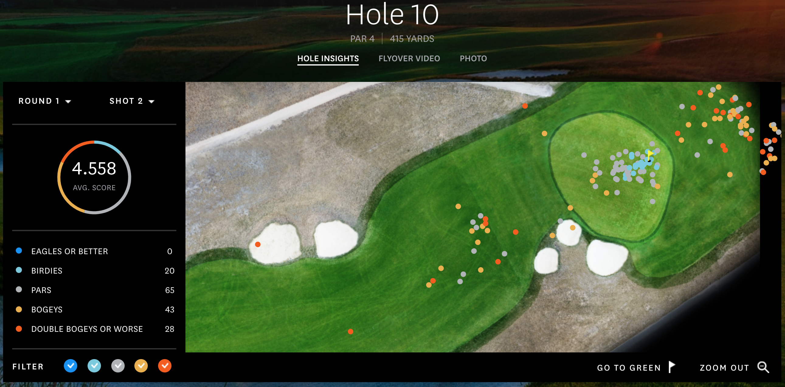
So this will be a second example of data for all the algorithms.

Algorithms themselves

This time, in this blog post, I’m only looking for results, not going through the algorithms themselves. There are other tutorials online talking about them, but for now at least, we’re only getting little introductions to the algorithms and thoughts.

Instead, I use the Scikit-Learn implementations of the algorithms. Scikit-Learn offers plenty of clustering algorithms, which I could spend hours using and writing about, but for this post, the ones I chose are K Means, DBSCAN, Mean Shift, Agglomerative Clustering.

Other Notes

Before going in to the algorithms, here are a few notes on what to expect.

  • Elevation is key as to why there are clusters. If you look around the other holes, you won’t see close to as much distribution and clusters of shot results. Now, if we had elevation as a data point as well, then we could really do some great cluster analyses.
  • The X and Y values on the sides of the graphs represent yards from the hole, which is located at the (0,0) location. If you look at the first post, I show that if you measure the hypotenuse using those X and Y numbers, you’ll have the yardage to the pin.
  • This isn’t a vast data set. We have 156 points in the two data sets because that’s how many players there were in the tournament.
  • If you’re wondering which part took the longest, it was writing the matplotlib code to automatically create figures with multiple plots for different input variables, and have them all show up at once. Presentation is key, and that took tons of time.

Code

I put all the code and data on Github here, so if you want to see what’s going on behind the scenes and what it took to do the analysis, look there.

Questions, comments, concerns, notes, thoughts, etc: contact, twitter, and golf twitter if you’re interested in that too. Ok, algorithm time.

K Means

I’m starting with K Means because this was the clustering algorithm I was first introduced to, and one that I had to write myself during a machine learning class in college.

Continue reading

U.S. Open Data — Gathering and Understanding the Data from 2018 Shinnecock

After losing in a playoff to make it out of the local qualifying for the 2018 US Open at Shinnecock, I’m stuck at my apartment watching everyone struggle, wondering how much I’d be struggling if I was there myself.

Besides on TV, the US Open website offers some other way to follow what players are doing. As shown here, they very generously give us information on everyone’s shots on different holes. We’re able to see where people hit the ball, on which shot, and what their resulting score was on the hole. For example, why in the world did Tony Finau, the currently second ranked longest hitter on tour, hit it short off the first tee, leave himself 230 yards to the hole where he makes bogey?

Why didn’t Tony rip D?

One of the cool things these images show is the groupings of all the shots on a hole, like the tee shots here. And when I see very specific and interactive data like we have here, I know it comes from somewhere that I’m able to see myself. So I figured I should grab that data and do some cluster analysis on different holes to see if there are certain spots that players like to hit it.

Here, I’ll go through the data we have, what the values and the numbers mean, and also the code I wrote to eat up the data and display the graphs. Once I have this part going, I’ll be able to perform further analysis to most things that come to mind.

Any questions, comments, concerns, trash talking, get in touch: twitter, contact.

Current Posts

Using Clustering Algorithms to Analyze Golf Shots

Finding the data

First step was to search for where the data for the hole insights page was coming from. As always, open the dev tools, click on the network tab, and find what’s getting called with a pretty name.

Alert!

The file itself is quite dense and has all the information, which is really cool! It has IDs for all the players, all the shots they have on the hole, which include the starting distance from the flag and the ending distance to the flag.

First off, we’re given a list of Ps, meaning an array of player information, like this:

...
{u'FN': u'Justin', u'ID': u'33448', u'IsA': False, u'LN': u'Thomas', u'Nat': u'USA', u'SN': u'THOMAS'},
{u'FN': u'Dustin', u'ID': u'30925', u'IsA': False, u'LN': u'Johnson', u'Nat': u'USA',u'SN': u'JOHNSON D'}
{u'FN': u'Tiger', u'ID': u'08793', u'IsA': False, u'LN': u'Woods', u'Nat': u'USA', u'SN': u'WOODS'}
...

It looks like we have first name, player’s ID, whether or not they’re an amateur, last name, nationality, scoreboard name. The important part of this information is the ID, where we’ll be able to match players to shots.

Next, we’re given a few stats on the hole for the day:

Continue reading

Talkin’ ‘Bout Trucks, Beer, and Love in Country Songs — Analyzing Genius Lyrics

Trucks, beer, and love, all things that make country music go round. I’ve said before that country music is just pop music with a slide, and then lyrics about slightly different topics than what you’ll hear in hip hop or “normal” pop music on the radio.

In my continuing quest to validate my theory that all country songs can fit into one of four different topics, in this post, I go through lyrics to see which artists talk about trucks, beer, and love the most. In my first post on this topic, I talked about how to get song lyrics from genius and print them out on the command line.

The goal here, and what I’m going to walk you through, is how I stored stored info and lyrics for all the songs for the country artists, how I made sure that all the lyrics were unique, and then ran some stats on the songs. Another note before we go is that a lot of data work is just janitorial. The actual code for getting “interesting” results is fairly simple. The key it to enjoy doing the janitor-style coding and then you’ll be good.

If you’re interested in which country music people talk most about trucks, beer, alcohol, or small towns, skip to the end where I list out some stats. For the rest, here’s some code.

https://www.pinterest.com/pin/59180182578213991/

I wonder how they feel about beer trucks. I’m guessing they’d all be fans of them.

Step 1 — Save the Lyrics!

When doing anything with web scraping, the one thing to always, always keep in mind here, is that you want to avoid hitting the server for as little as possible. With that in mind, we’re going to do here is assume the inputs are names of artists. For each of those artists, find all of their songs, and then for each of those songs, grab the lyrics in the way that I did in the first post, and then save them locally along with some meta information the API provides.

Now when I post the following code, don’t imagine that I knew what I wanted . Everything in here was created iteratively. Here’s a list of all the features of this piece of code does that were created iteratively.

Directory structure — Within the folder that contains the main .py file, there’s a folder named artists. And within that folder, when the code runs, a folder with the artist’s name is created (if not already). And within that folder, there are two more folders, info and lyrics. When we run the code, I put the lyrics in /artists/artist_name/lyrics/Song Title.txt and the info from the API, containing information about the song, like annotations, title, and song API id so we can grab it again if need be, in the file /artists/artist_name/info/Song Title.txt. The key, again, being saving all the info given to avoid unnecessary requests.

Redundancy Checking — Along with making sure to save all the info given, if we run an artist for the second time, we don’t want to get lyrics that we already have. So once we have all the songs for that artist, I run a check to see if we have a file with the name of the song already, and that the file isn’t empty. If the file is there, we continue to the next song.

Lyric Error Checking — Ahh unicode. While great for allowing multitudes of different characters rather than the standard English alphabet along with a few specialty characters, they’re not ideal when I’m trying to deal with simple song lyrics. And when saving the lyrics, I encountered more than a few random, unnecessary characters that Python threw errors for encoding problems. In a semi-janky rule-based solution (which isn’t great to use, see below), when I saw these errors being thrown, I would specifically replace them with the correct “normal” character. I assume there’s some library out there that would take care of all the encoding issues, but this worked for me. Also, on Genius’s end, it would be sweet if they, you know, checked for abnormal characters when lyrics were uploaded and didn’t have them in the first place. Also would be cool if they included the lyrics in the API.

def clean_lyrics(lyrics):
  lyrics = lyrics.replace(u"\u2019", "'") #right quotation mark
  lyrics = lyrics.replace(u"\u2018", "'") #left quotation mark
  lyrics = lyrics.replace(u"\u02bc", "'") #a with dots on top
  lyrics = lyrics.replace(u"\xe9", "e") #e with an accent
  lyrics = lyrics.replace(u"\xe8", "e") #e with an backwards accent
  lyrics = lyrics.replace(u"\xe0", "a") #a with an accent
  lyrics = lyrics.replace(u"\u2026", "...") #ellipsis apparently
  lyrics = lyrics.replace(u"\u2012", "-") #hyphen or dash
  lyrics = lyrics.replace(u"\u2013", "-") #other type of hyphen or dash
  lyrics = lyrics.replace(u"\u2014", "-") #other type of hyphen or dash
  lyrics = lyrics.replace(u"\u201c", '"') #left double quote
  lyrics = lyrics.replace(u"\u201d", '"') #right double quote
  lyrics = lyrics.replace(u"\u200b", ' ') #zero width space ?
  lyrics = lyrics.replace(u"\x92", "'") #different quote
  lyrics = lyrics.replace(u"\x91", "'") #still different quote
  lyrics = lyrics.replace(u"\xf1", "n") #n with tilde!
  lyrics = lyrics.replace(u"\xed", "i") #i with accent
  lyrics = lyrics.replace(u"\xe1", "a") #a with accent
  lyrics = lyrics.replace(u"\xea", "e") #e with circumflex
  lyrics = lyrics.replace(u"\xf3", "o") #o with accent
  lyrics = lyrics.replace(u"\xb4", "") #just an accent, so remove
  lyrics = lyrics.replace(u"\xeb", "e") #e with dots on top
  lyrics = lyrics.replace(u"\xe4", "a") #a with dots on top
  lyrics = lyrics.replace(u"\xe7", "c") #c with squigly bottom
  return lyrics

Check out the most of the main function below. If you’re looking for the actual full file, check out this gist. It’s easier to post that on Github than formatting the entire thing here.

Continue reading

Python, Postgres, SQLAlchemy, and PGA Tour Stats

A little ago, I wrote an article about scraping a bunch of PGA Tour stats. The end result of that was writing those stats out into CSV files. While this was suitable for that task of gathering the stats, let’s face it, you’re probably going to want to put those into some database to allow for easier querying, or possibly integrate it into to web app in the future. There are a bunch of different reasons for wanting this, so I’m going to go through the process I took to put all the data in the CSV files into the database.

Adding players to the database

First step is to fire up postgres! I’m not going to cover starting postgres since there’s so much good content about it, for example, this super good tutorial here by Digital Ocean. I created at database called ‘pgatour’, created a user named ‘pgatour_user’ with password ‘pgatour_user_password’, logged in, and created the first table, Player.

pgatour=# create table players (
  id serial PRIMARY KEY,
  name varchar (255) NOT NULL
);

Ok, now, as a test, I’m going to add myself into the database from the psql command line.

pgatour=# insert into players (name) values ('Jack Schultz')

Note that since id is serial, we don’t need to insert that value, just the name. Alas, I am not on the PGA Tour, so I’m going to need to delete myself.

pgatour=# select * from players;
id | name
----+--------------
1 | Jack Schultz
(1 row)

pgatour=# delete from players where name = 'Jack Schultz';
DELETE 1
pgatour=# select * from players;
id | name
----+------
(0 rows)

Looking good. Now onto the Python side.

Python SQL Alchemy Interface

Now that the Players table in the database is set up, we’re going to want to be able to modify the contents of it in Python.

Continue reading

What’s the Average Age of a Nobel Prize Winner?

tl;dr —  Average age of a Noble Prize winner is 59.14 years old.

There was a comment on HN the other day about wondering about the average age of Nobel Prize winners. I did a quick search for lists of Nobel Prize winners, and the Nobel Prize org’s website actually has a page listing winners and their ages. The data’s tucked in the html file, but I figured with scraping and a little numerical work, I could do a little analysis easily.

The first thing I did was download that html file, and store it locally. Sure I’m scraping data from an html file, but there’s no reason for me to hit the server every time I’m testing / adjusting my script. It’s important to realize that even though I’m dealing with a web page, I don’t have to actually use the internet to do the analysis. Downloading the page simplifies things on my end by not having to use the requests library, and also saves a few server hits on the other end.

The other thing it allows me to do is modify the html and put an id on a div tag which helps me locate the data I want. After look through, the div that contained all the data about the winners and their ages didn’t have a class, id, or anything else identifiable. It was literally just a div tag, and when you’re trying to automate data collection from a DOM, classes and ids are key. But since I downloaded the page, I was able to put an id on the div I needed to grab, and didn’t have to deal around with maneuvering to it using parent tags.

The relevant info for each of the winners was structured pretty well within that div. In order to organize the information, I created a class for each of the prize winners, and input the data by looping through the html.

class Prize:
 def __init__(self, name, age, year, prize_type):
 self.name = unicodedata.normalize('NFKD', name).encode('ascii','ignore') #umlaut issues
 self.age = age
 self.year = year
 self.prize_type = prize_type

 def __str__(self):
   return self.name + ' won ' + str(self.prize_type) + ' at age ' + str(self.age) + ' in ' + str(self.year)

f = open('nobel_laureates_by_age.html', 'r')
html = BeautifulSoup(f.read())

winners = []
prize_types = set()
nobel_prize_string = "The Nobel Prize in "
for tag in html.find("div", id="nobel-age-info").children:
  # we're looking for a specific div, that doesn't have a class, id, or anything noteworthy
  #so I'm going to count the divs that are in this outerdiv until we hit the one I want
  if tag.name == None:
    next
  elif tag.name == 'h3':
    current_age = int(tag.text.split(" ")[-1]) #update the age
  elif tag.name == 'div':
    name = tag.find("h6").text #winner's name
    description = tag.find_all("p")[0].find("a").text #winner's name
    year = int(description.split(' ')[-1])
    prize_type = ' '.join(description.split(' ')[0:-1])
    prize_types.add(prize_type)
    prize = Prize(name, current_age, int(year), prize_type, description)
    winners.append(prize)

From here, we want to get an average and a visualization of the ages of the winners for each prize.

all_prize_string = "All Prizes"
ts = list(prize_types)
ts.append(all_prize_string) #want to get all prizes too

print "Type, Number of Winners, Mean Age, Variance of Ages"
for prize_type in ts:
  ages = [p.age for p in winners if p.prize_type == prize_type or prize_type == all_prize_string]
  num_bins = ages[-1] - ages[0]
  fig = plt.figure()
  n, bins, patches = plt.hist(ages, num_bins, normed=1, facecolor='green', alpha=0.2)
  mean, var = norm.fit(ages)
  y = mlab.normpdf(bins, mean, var)
  plt.plot(bins, y, 'r--')
  plt.ylabel('Number of Winners')
  plt.xlabel('Age')
  plt.title(prize_type + '. Mean: ' + str(round(mean,2)) + ', Var: ' + str(round(var,2)))
  fig.savefig('nobel_hist_' + prize_type.lower().replace(' ', '_') + '.png', dpi=500,format='png')
  print prize_type +', '+ str(len(ages)) +', '+ str(round(mean,2)) +', '+ str(round(var,2))

The code above print out a little csv table for each of the prize types, as well as creating a histogram and fitted distribution for each, as well as the ages for everyone, regardless of prize type.

Somewhat grainy images of the fits are below

nobel_hist_all_prizes

nobel_hist_the_prize_in_economic_sciences

nobel_hist_the_nobel_prize_in_physiology_or_medicine

nobel_hist_the_nobel_prize_in_physics

nobel_hist_the_nobel_prize_in_chemistry

nobel_hist_the_nobel_prize_in__literature

nobel_hist_the_nobel_peace_prize

Some Thoughts

The overall age distribution is impressively normal. The couple outliers on the younger side are the 2014 Peace Prize winner Malala Yousafzai, and the 1915 Physics winner William Lawrence Bragg who won jointly with his father for work with X-Rays. Besides those winners, the rest seem pretty centered around the 60 year old mark.

There’s a funny dip in the graph for the prize on literature right around the mean. Only one winner with an age of 64-66. Funny because the mean for that award is about 65.

Youngest winners for each:

Chemistry: 35
Literature: 42
Peace: 17
Physiology or Medicine: 32
Economics: 51

Oldest Winners for Each

Chemistry: 85
Literature: 88
Peace: 87
Physiology or Medicine: 87
Economics: 90
Physics: 88

Oldest winners seem to be around the same age, while the younger winners seem to differ by prize type. Kind of interesting, given that the prize for Economics wasn’t started by Nobel in 1895 like the others, but rather in 1969. (Check out the wikipedia entry here.) The fewer number of winners could explain the youngest winner outlier. Once the award has been around for longer, you’d expect someone younger than 51 to win. Using the distributions, we can actually guess the probability that someone younger than 51 will win: about 2.5%.

Another explanation that I’ve heard before is that sometimes prizes are won for contributions over time. They want to recognize a person for their contributions over their careers, but not necessarily their research in their winning year. That could easily push the average age up. Obviously the Nobel Foundation would refute that, but who knows.

Possible Continuations

NLP on the descriptions — Most of the winner’s have a little sentence below that talks about what they did to deserve the prize. Some processing on that text might be interesting, like seeing what the popular keywords are for example.

Deal with multiple people sharing the prize — The reason there are over 800 winners of the 6 prizes is because people share the prize. The links on the page go to a more full description of the prize winner(s). For shared prizes, I might want to take the average age for the winners and only use that. I could also do an analysis on how often the prize is shared as opposed to won outright. Maybe the percentage of shared awards have changed over time?

Check out the gist here. Requires that you download the html like and add the id to the tag like mentioned above. And also have the required libraries installed with pip.

Comments? Want further analysis? Want to yell at me for bad analysis? Let me know on twitter.