NPR Sunday Puzzle Solving, And Other Baby Name Questions

Posted on October 2, 2017 by Jack Schultz

If you have a long drive and no bluetooth or aux cord to listen to podcasts, NPR is easily the best alternative. Truck drivers agree with this statement no matter their overall views. For me, this was the case when driving home to Milwaukee from Ann Arbor where I went to a college friend’s wedding.

While driving back I listened to NPR and heard Weekend Edition Sunday and their Sunday Puzzle pop up. If you haven’t heart of it before, at the end of every week’s episode they state a puzzle. Throughout the next week listeners can submit their answer and one random correct submitter is chosen to be recorded doing a mini puzzle on air.

The puzzle they stated for the week after the wedding was as follows:

Think of a familiar 6-letter boy’s name starting with a vowel. Change the first letter to a consonant to get another familiar boy’s name. Then change the first letter to another consonant to get another familiar boy’s name. What names are these?

They’ve already released the show for this question (I didn’t win of course) so I figure I can write about how I found out the answer!

Solving The Name Question

First step as always for these types of posts is gathering the required list of familiar boy’s names. Searching on Google for lists will show that there are a ton of sites which exist try to SEO themselves for the money. When scraping, you should to poke around and make sure to choose the post that has the correct data as well as being the most simple to gather. I went with this one.

Since there’s only one page with the data, there’s no need to use the requests library to scrape the different pages. So clicking save html file to the folder you’re programming in is the best way to get the data.

The scraping code itself is pretty simple.

from bs4 import BeautifulSoup

filename = 'boy_names.html'
vowels = ('A', 'E', 'I', 'O', 'U')

vowel_starters = []
consonant_starters = []

with open(filename, 'r') as file:
  page = file.read()
  html = BeautifulSoup(page.replace('\n',''), 'html.parser')
  for name_link in html.find_all("li", class_="p1"):
    name = name_link.text
    first_letter = name[0]
    if len(name) == 6:
      if first_letter in vowels:
        vowel_starters.append(name)
      else:
        consonant_starters.append(name)

for vname in vowel_starters:
  cname_same = []
  for cname in consonant_starters:
    if vname[1:] == cname[1:]:
      cname_same.append(cname)
  if cname_same:
    print vname
    for match in cname_same:
      print match

And the results are…

Austin, Justin, Dustin

Justin and Dustin rhyme which makes it more simple to realize that they match, but Austin isn’t exactly on the same page. If I didn’t have the code, zero chance I’d have gotten this correct.

That’s it right? Nope, I have all the code, I figured I should check to see if there’s a match for girls names with that same rules. All there was to do is save the popular girl names to the same folder, change the filename to ‘girl_names.html’, run the code, and we’ll get Ariana and Briana. A and B are the starting letters, and if Criana was a popular name (at this moment), we’d be good to for the full 3 name answers.

By going through this part, I came up with some other fun questions that could be answered with this list of names, and the rest of the post is about those.

Continue reading →

Getting Song Lyrics from Genius’s API + Scraping

Posted on September 27, 2016 by Jack Schultz

Genius is a great resource. At a high level, Genius has song lyrics and allows users to comment on what the artist meant. Starting as Rap Genius, where users annotated rap lyrics, the site rebranded as “Genius”, allowing all songs to be talked about. According to their website, “Genius is the world’s biggest collection of song lyrics and crowdsourced musical knowledge.” Recently even, they’ve moved to allowing annotations of pretty much anything posted online.

I’ve have used it a bunch recently while trying to figure out what the hell Frank Ocean was trying to say in his new album Blond. Users of the site explained tons of Frank’s references that went whoosh right over my head when I listened the first time and all the times after.

And recently, when I had some ideas for mini projects using song lyrics, I was pretty happy to find that Genius had a API for getting the data on their site. Whenever I’m trying to get data elsewhere, I’m much happier with an API, or at least being able to get it from JSON responses rather than parsing HTML. It’s just cleaner to look at, and with an API, I can expect good documentation that isn’t going to change with css updates.

Their API docs looked pretty good at first glance, with endpoints for artists, songs, albums, and annotations. One things I did notice was that they don’t have an artist entry point. A lot of what I want to do is artist based, meaning I need to know the artist id for everyone. And in order for me to get that, I have to search the artist, grab a song from the results, hit the song endpoint for that song’s information, and then grab the artist id from there. It’d be nice if you could specify what I’m searching for when I hit the search endpoint so I don’t have to go through that whole charade just to get the artist. But that’s a blog post for another time. Overall, they give out tons of information pretty easily.

But why, Genius, why don’t you have an endpoint for getting the raw lyrics of a song?! You have a songs endpoint on the API, and you give me a ton of information from there — the song title, album name, featured artists on the song, number of annotations, images associated with the song, album information, page views for that song, and a whole host of more data. But the one thing you don’t give me, and the one thing that people using the API probably want the most, is plain text lyrics!

Pre-Genius, I was stuck with these jankily laid out sites with super old looking css that would have the lyrics, but not necessarily correct, and definitely no annotations. Those sites are probably easily scrapeable considering their simplicity, but searching for the right song would be more difficult, and the lyrics might not be correct. Genius solved this all now for a web user, but dammit, I want the lyrics in the API!

Now you might be able to get the entire set of lyrics by using the annotations endpoint, which had information about all the annotations for a certain song or article, but that would require a song to have annotations for every word in the song. For someone like Chance the Rapper who like Frank Ocean (and most other hip hop artists uses tons of references in his lyrics, having complete annotations might not be an issue. But of Jake Owen, who’s new single “American Country Love Song” has probably the most self explanatory lyrics ever (sorry for throwing you under the bus here, Jake. Still a fan), there’s no need to annotate anything, and getting the lyrics in this manner wouldn’t work.

The lyrics are there on the internet however, and I can get at them by hitting the song endpoint, and using the web url that it returns. The rest of this article will show you how to do that using Python and it’s requests and BeautifulSoup libraries. But I don’t have to have to resort to HTML parsing, and I don’t think Genius wants users doing that either.

I’m left here wondering why they don’t want to give up the lyrics so easily, and I really don’t have much to go on. Genius’s goal seems to be wanting to annotate the internet. It has already moved on from their initial site of Rap Genius, into all music, and now into speech transcripts, as well as pretty much any other content on the web. Their value comes from those annotations themselves, not the information they’re annotating. They give away the annotations freely, but not the information (lyrics) in this case.

Enough speculation on why Genius doesn’t spit out the lyrics to a song when you get the other information. And as I’m writing this, I realize I easily could have overlooked something in their API and Genius might return the full lyrics, but I overlooked it. In that case, half of this article will be pointless and I’ll hold my head in shame from yelling at them like I did.

For purposes here, I’m going to show you how to get the song lyrics from Genius if you have the song title, and also talk through my process of getting there.

Note of clarification, just to make sure I’m not violating their terms of service, this post is for informational purposes only. Hopefully this can help programmers out there learn. Don’t do something bad with this knowledge. Code time!

First thing you’re going to need is an account set up with Genius. You can sign up from the upper right hand corner of the genius.com homepage. After that, navigate to the api docs where you’ll then see your Bearer token that you’ll need for all API requests.

I’m using the requests library here, and once you have the bearer token, here’s what all the API requests to Genius should look like if, for example, you’re searching for a song title.

import requests

#TOKEN below should be the string that the API docs tells you
#Clearly I'm not giving mine out here on the internet. That'd be dumb
base_url = "http://api.genius.com"
#Key line below here when, this is how to authorize your request when
#using the API
headers = {'Authorization': 'Bearer TOKEN'}
search_url = base_url + "/search"
song_title = "In the Midst of It All"
params = {'q': song_title}
response = requests.get(search_url, params=params, headers=headers)

The response, according to the Genius API, would be a list of songs that match that string passed in, with the first result being the Tom Misch song that I was going for. By changing around the url that is passed into the request method, you can access all the information that Genius supplies from the API (pretty much everything but the lyrics).

Continue reading →

The Special Relationship Between Noodles and Qdoba

Posted on May 3, 2016 by Jack Schultz

I’ve had a theory that for every Noodles, there’s a Qdoba that’s right next door. It might be some sort of selection bias however, since I can think of a couple locations where they’re directly next to each other. To me, Noodles and Qdoba have a special relationship, at least compared to other restaurants. I figured now was about the time I should test this, and I can use Chipotle to test.

The question is: Which restaurant is more special to Noodles, Qdoba or Chipotle?

Finding the Noodles, Qdoba, and Chipotle locations

Initially, I went to Noodle’s website and their locations page and was planning on getting the data from there. But what I realized was that it just used the Google Maps API to get it’s data, so I might as well just go right to the Google source and use their api correctly.

Google’s docs are pretty good in this case, and after grabbing an API key, I started in on finding the Dobas. For prototyping, I just started with the latitude and longitude of Milwaukee, my home town, and a place where I know there multiple Qdobas / Noodles pairs.

import requests
url = 'https://maps.googleapis.com/maps/api/place/nearbysearch/json'
location_milwaukee = '43.0389,-87.9065' #Milwaukee
params = {}
params['key'] = GOOGLE_PLACES_API
params['type'] = 'restaurant'
params['radius'] = 50000 #in meters, and going be an issue
params['keyword'] = 'Qdoba'
params['location'] = location
r = requests.get(url, params=params)
results = r.json()['results']
print results

Put your Google Places API key in the ‘key’ param, run those lines of code (assuming you pip installed requests) and you’ll see 20 Qdoba locations along with some extra information spit out on your console.

Issues

Two obstacles came up with this part of the project – one simple to fix, the other decently tough. First the simple one.

In order to limit the amount of information coming across the wire, Google limits each API request to 20 results. When there are more than 20 results they find, they also pass back in the json a param named “next_page_token”. So when we see this param passed back, we need to stick with the same location, and add the param “pagetoken” and hit the same endpoint. There’s also a time aspect to this request where we need to wait a couple seconds before hitting the endpoint to grab the remaining locations. Not too bad.

Second issue here, and somewhat of an annoying one, is the radius parameter. 50 km is not quite the size of the entire US. This is actually a really interesting problem that, after talking with work colleagues, there isn’t a straightforward solution. What we really need here, is a set of latitudes and longitudes where, with the 50 km radius, will cover the entirety of the United States. Sure you could put a location every miles or so, but that would take forever to search for. So instead of finding a solution to this problem isn’t in the scope of this article (maybe later). Instead, I found this nice gist of the top 246 metro locations in the US and their latitude and longitudes and am just going to use that and hope it covers enough of the country to be useful.

Complete code for this part of the project includes writing the locations of the restaurants to a tab separated values (tsv) file. Normally would use a csv, but since the addresses have commas in them, it could get confusing.

from major_city_list import major_cities

keyword_qdoba = 'Qdoba Mexican Eats'
keyword_noodles = 'Noodles & Company'
keyword_chipotle = 'Chipotle'
search_keywords = [keyword_qdoba, keyword_noodles, keyword_chipotle]

params = {}
params['key'] = GOOGLE_PLACES_API
params['type'] = 'restaurant'
params['radius'] = 50000
for keyword in search_keywords:
  params['keyword'] = keyword
  keyword_info = {}
  for city in major_cities:
    print city["city"]
    location = "%s,%s" % (city["latitude"], city["longitude"])
    params['location'] = location
    while True:
      r = requests.get(url, params=params)
      results = r.json()['results']
      num_results = len(results)
      print "results: %s" % num_results
      for result in results:
        lat = result["geometry"]["location"]["lat"]
        lng = result["geometry"]["location"]["lng"]
        key = "%s%s" % (lat, lng * -1)
        address = result["vicinity"]
        info = {"lat": lat, "lng": lng, "address": address}
        keyword_info[key] = info
        try:
          next_page_token = r.json()['next_page_token']
          params["pagetoken"] = next_page_token
          time.sleep(2)
        except KeyError:
          params.pop("pagetoken", None)
          break

 filename = "%s.tsv" % keyword
 filename = filename.lower().replace(" ", "_")
 with open(filename, 'wb') as tsvfile:
   writer = csv.writer(tsvfile, delimiter='\t')
   for key, info in keyword_info.iteritems():
     writer.writerow([info['lat'],info['lng'],info['address']])

Final thing to point out here is about why I have this be a multi step process. I could have written a script that does this part, and then all the rest of the project at once. But you’ll find that when working on things and bugfixing, it’s better to split tasks up, save the results, and then use those results without having to go back out to the internet.

Finding nearest companion

Step two of this process here is finding the closest Qdoba and Chipotle for each Noodles. With that information, we can figure out how far away the nearest companion is. At first, I was tempted to go right back to the Google Places API since, well, it was designed for this purpose. However first, I decided to see if I could brute force it with the n^2 loop over every location and find the shortest distance algorithm. Turns out that was a great decision because it was way quicker and more accurate.

Code steps are 1) Read in the noodles.tsv file generated above, 2) read in the chipotle and qdoba .tsv files, 3) for each Noodles, loop the entire other file and store the closest location, 4) store that information in another tsv file. In this case, code is easier to figure out than explanation.

keywords = ['chipotle', 'qdoba']
noodles_locations = []
filename = "noodles.tsv"
with open(filename, 'rb') as tsvfile:
  reader = csv.reader(tsvfile, delimiter='\t')
  for row in reader:
    noodles_locations.append(row)
for keyword in keywords:
  information = []
  filename = "%s.tsv" % keyword
  keyword_locations = []
  with open(filename, 'rb') as tsvfile:
    reader = csv.reader(tsvfile, delimiter='\t')
    for row in reader:
      keyword_locations.append(row)
  count = 0
  for noodle_location in noodles_locations:
    print count
    test_loc = (noodle_location[0], noodle_location[1])
    best_distance = 100000 #something large
    for location in keyword_locations:
      found_loc = (location[0], location[1])
      distance = vincenty(test_loc, found_loc).miles
      if distance < best_distance:
        best_distance = distance
        best_location = [location[0], location[1], location[2]]
    info_row = [noodle_location[0], noodle_location[1], noodle_location[2], best_location[0], best_location[1], best_location[2]]
    information.append(info_row)
    count += 1
    filename = "noodles_closest_%s.tsv" % keyword
    with open(filename, 'wb') as tsvfile:
      writer = csv.writer(tsvfile, delimiter='\t')
      for info in information:
        writer.writerow(info)

Analyze!

For my dumb theory to be true, there needs to be a disproportionate number of Qdobas and Noodles within walking distance of each other, and specifically, right next to each other compared to Chipotle.

After analyzing the data, I’m totally right.

I found 418 Noodles, 790 Chipotles, and 618 Qdobas. Even with the extra 172 Chipotles, there’s a Qdoba closer to a Noodles than there is a Chipotle.

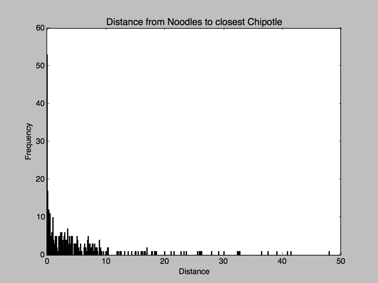
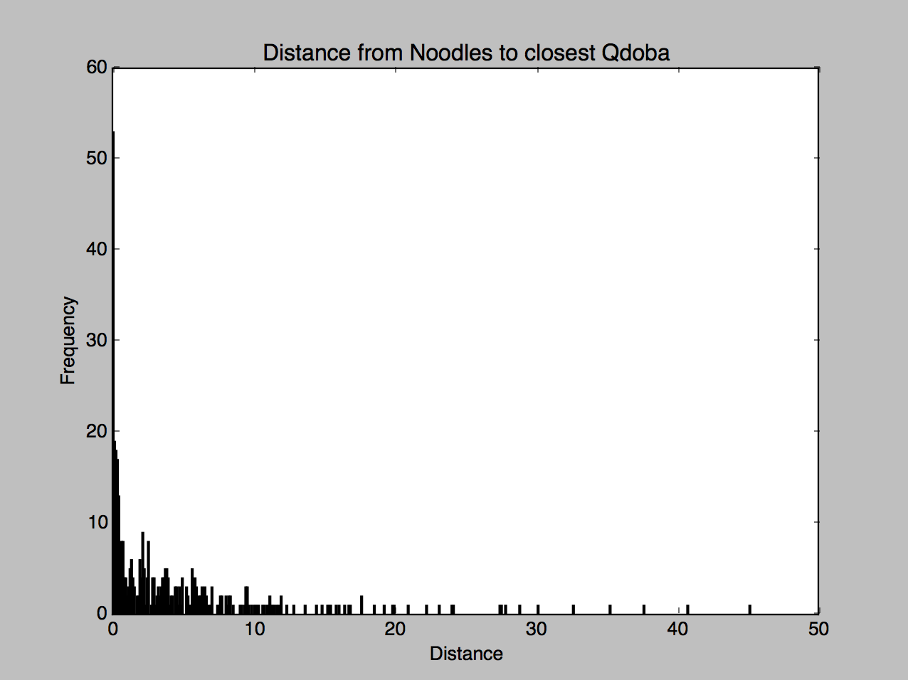
Some numbers. If you’re at a Noodles, there’s a 12.7% chance you’re within 0.1 miles of a Qdoba, 19.9% chance you’re within 0.25 miles, and 35.9% chance you’re within 1 mile. Chipotle has percentages of 6.4%, 12.7%, 30.6% respectively.

Check out the histograms:

While not much of a difference, you can see a little more action on the left side of the Qdoba histogram compared to the Chipotle one.

As a final, final test, I went through each Noodle location again, found the nearest Qdoba and nearest Chipotle and counted the number of Noodles that had a Qdoba closer, and Noodles that had Chipotle closer. Final tally, 214 had a Qdoba closer, 204 had a Chipotle closer.

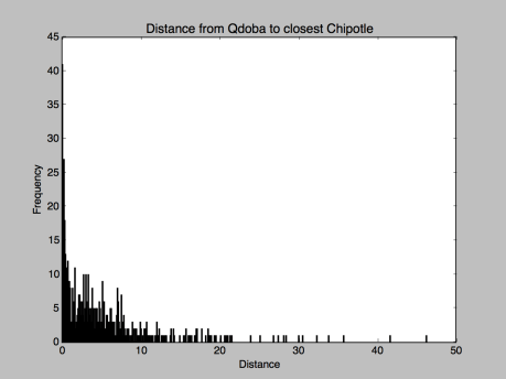
So how close are Qdobas and Chipotles from each other?

For fun, I ran the code to see how close the nearest Chipotle was from each Qdoba.

6.6% Qdobas had a Chipotle within 0.1 miles, 12.8% had one within 0.25 miles, and 28% within 1 mile. Semi-surprising that it was this high, but I guess people don’t want to go far for food.

The histogram is definitely more telling that Chipotles are further apart. Check out the y axis scaling here.

What’s the point of this?

Knowing this kind of information really isn’t all that useful. Fun, sure, but not too particularly useful. But what it does show is how powerful knowledge of the internet and programming can be. In just a short amount of time, we went from a dumb theory about restaurants to finding an answer. Also, maybe you’re looking to open a Qdoba somewhere in the US, and want to know if there’s a lonely Noodles that needs a companion!

Follow on twitter, and get in contact if you have information you want on the internet. I can help you out!

Gather all the PGA Tour stats

Posted on March 5, 2016 by Jack Schultz

As someone who likes writing and investigating data sets, and as a huge fan of golf (and writer of a golf blog, Golf on the Mind), when I realized that the PGA Tour website has a crap ton of stats about players on the PGA Tour going back to the early 80s, I figured there was definitely some investigating to do. And the first step, as with any data analysis, is getting the data into a standard and usable form. And in reality, you’ll find this effort takes up most of your time if you do this sort of thing.

So before I can start looking at anything interesting, I need to do some scraping. This article will take you through that process.

UPDATE — 5/25/18 — I get way too many questions about whether the data is available, so I went back through and updated the code and currently scraping it every week. I’m not going to post the link here, but shoot me an email and I can go ahead and share the links.

Step 1 — Downloading the HTML files

The usual process for scraping, is to grab the html page, extract the data from that page, store that data. Repeat for however many web pages have the data you want. In this case however I wanted to do something different. Instead of grabbing the data from a web page and storing that data, I wanted to actually store the html file itself as a first step. Only after would I deal with getting the info from that page.

Reasoning behind this was to avoid unnecessarily hitting pgatour.com’s servers. Undoubtedly, when scraping, you’ll run into errors in your code – either missing data, oddly formatted data you didn’t account for, or any other random errors that can happen. When this happens, and you have to go back and grab the web page again, you’re both wasting time by grabbing the same file over the internet, and using up resources on that server’s end. Neither a good result.

So in my case here, I wrote code to download and save the html once, and then I can extract data as I please from those files without going over the internet. Now for the specifics.

On pgatour.com, the stats base page is located at pgatour.com/stats.html. If you notice at the top. This will land you at the overview page, but you can notice at the top there are eight categories of stats: Off the Tee, Approach the Green, Around the Green, Putting, Scoring, Streaks, Money/Finishes, and Points/Rankings. Under each of these categories are a list of stats in a table. Clicking on any of those links and you’ll get the current year’s stats for all the qualifying players. On the side, you’ll notice a dropdown where you can select the year you want the stat for. Our goal is to get the pages for each of those stats, for every year offered, and save the page in a directory named for the stat, and the year as the filename.

The url pattern when you’re on a single stat is straight forward. For example the url for current Driving Distance is http://www.pgatour.com/stats/stat.101.html, and the url for Driving Distance in 2015 is http://www.pgatour.com/stats/stat.101.2015.html. Simply injecting the year into the url after the stat id will get you what you need.

In order to get the different stats from the category page, we’re going to loop the categories, yank out url and name for a stat, grab the current page, see which years the stat is offered for, generate the required urls, and loop those urls saving the page! Reading the code should make this make more sense.

The last issue with grabbing the html pages is how long it takes. In the end, we’re talking about over 100 stats, with about 15-20 years of history. At first, I wanted to play nice not overwhelm the pgatour.com servers, but then I realized that pgatour.com can probably handle the load since they need to be able to deal with the constant refreshing that people do when checking leaderboards at the end of a tournament. Thankfully, python’s Gevent library allows us to easily, in parallel, grab pages and save them. After all that explanation, take a look at the code I used to save the files.

url_stub = "http://www.pgatour.com/stats/stat.%s.%s.html" #stat id, year
category_url_stub = 'http://www.pgatour.com/stats/categories.%s.html'
category_labels = ['RPTS_INQ', 'ROTT_INQ', 'RAPP_INQ', 'RARG_INQ', 'RPUT_INQ', 'RSCR_INQ', 'RSTR_INQ', 'RMNY_INQ']
pga_tour_base_url = "http://www.pgatour.com"
def gather_pages(url, filename):
 print filename
 urllib.urlretrieve(url, filename)

def gather_html():
 stat_ids = []
 for category in category_labels:
 category_url = category_url_stub % (category)
 page = requests.get(category_url)
 html = BeautifulSoup(page.text.replace('\n',''), 'html.parser')
 for table in html.find_all("div", class_="table-content"):
   for link in table.find_all("a"):
     stat_ids.append(link['href'].split('.')[1])
 starting_year = 2015 #page in order to see which years we have info for
 for stat_id in stat_ids:
   url = url_stub % (stat_id, starting_year)
   page = requests.get(url)
   html = BeautifulSoup(page.text.replace('\n',''), 'html.parser')
   stat = html.find("div", class_="parsys mainParsys").find('h3').text
   print stat
   directory = "stats_html/%s" % stat.replace('/', ' ') #need to replace to avoid
   if not os.path.exists(directory):
     os.makedirs(directory)
   years = []
   for option in html.find("select", class_="statistics-details-select").find_all("option"):
     year = option['value']
     if year not in years:
       years.append(year)
   url_filenames = []
   for year in years:
     url = url_stub % (stat_id, year)
     filename = "%s/%s.html" % (directory, year)
     if not os.path.isfile(filename): #this check saves time if you've already downloaded the page
       url_filenames.append((url, filename))
     jobs = [gevent.spawn(gather_pages, pair[0], pair[1]) for pair in url_filenames]
     gevent.joinall(jobs)

Step 2 — Convert HTML to CSV

Now that I have the html files for every stat, I want to go through the process of getting the info from the tables in the html, into a consumable csv format. Luckily, the html is very nicely formatted so I can actually use the info. I saved all the html files in a directory called stats_html, and I basically want to create the same folder structure in a top level directory I’m calling stats_csv.

Steps in this task are 1) Read in the files, 2) using Beautiful Soup, extract the headers for the table, and then all of the data rows and 3) write that info as a csv file. I’ll just go right to the code since that’s easiest to understand as well.


for folder in os.listdir("stats_html"):
 path = "stats_html/%s" % folder
 if os.path.isdir(path):
   for file in os.listdir(path):
   if file[0] == '.':
     continue #.DS_Store issues
   csv_lines = []
   file_path = path + "/" + file
   csv_dir = "stats_csv/" + folder
   if not os.path.exists(csv_dir):
     os.makedirs(csv_dir)
   csv_file_path = csv_dir + "/" + file.split('.')[0] + '.csv'
   print csv_file_path
   if os.path.isfile(csv_file_path): #pass if already done the conversion
     continue
   with open(file_path, 'r') as ff:
     f = ff.read()
     html = BeautifulSoup(f.replace('\n',''), 'html.parser')
     table = html.find('table', class_='table-styled')
     headings = [t.text for t in table.find('thead').find_all('th')]
     csv_lines.append(headings)
     for tr in table.find('tbody').find_all('tr'):
       info = [td.text.replace(u'\xa0', u' ').strip() for td in tr.find_all('td')]
     csv_lines.append(info)
     #write the array to csv
     with open(csv_file_path, 'wb') as csvfile:
       writer = spamwriter = csv.writer(csvfile, delimiter=',')
       for row in csv_lines:
         writer.writerow(row)

And that’s it for the scraping! There are still a couple issues before you can actually use the data, but those issues are dependent on what you’re trying to find out. The big example being getting the important piece of info from the csv. Some of the stats are percentage based stats, others are distance measured in yards. There are also stats measured in feet / inches (23’3″ for example). Also an issue is that sometimes, the desired stat is in a different column in the csv file depending on the year the stat is from. But like I said, those issues aren’t for an article on data scraping, but we’ll have to deal with them when looking at the data later.

What’s the Average Age of a Nobel Prize Winner?

Posted on June 7, 2015 by Jack Schultz

tl;dr — Average age of a Noble Prize winner is 59.14 years old.

There was a comment on HN the other day about wondering about the average age of Nobel Prize winners. I did a quick search for lists of Nobel Prize winners, and the Nobel Prize org’s website actually has a page listing winners and their ages. The data’s tucked in the html file, but I figured with scraping and a little numerical work, I could do a little analysis easily.

The first thing I did was download that html file, and store it locally. Sure I’m scraping data from an html file, but there’s no reason for me to hit the server every time I’m testing / adjusting my script. It’s important to realize that even though I’m dealing with a web page, I don’t have to actually use the internet to do the analysis. Downloading the page simplifies things on my end by not having to use the requests library, and also saves a few server hits on the other end.

The other thing it allows me to do is modify the html and put an id on a div tag which helps me locate the data I want. After look through, the div that contained all the data about the winners and their ages didn’t have a class, id, or anything else identifiable. It was literally just a div tag, and when you’re trying to automate data collection from a DOM, classes and ids are key. But since I downloaded the page, I was able to put an id on the div I needed to grab, and didn’t have to deal around with maneuvering to it using parent tags.

The relevant info for each of the winners was structured pretty well within that div. In order to organize the information, I created a class for each of the prize winners, and input the data by looping through the html.

class Prize:
 def __init__(self, name, age, year, prize_type):
 self.name = unicodedata.normalize('NFKD', name).encode('ascii','ignore') #umlaut issues
 self.age = age
 self.year = year
 self.prize_type = prize_type

 def __str__(self):
   return self.name + ' won ' + str(self.prize_type) + ' at age ' + str(self.age) + ' in ' + str(self.year)

f = open('nobel_laureates_by_age.html', 'r')
html = BeautifulSoup(f.read())

winners = []
prize_types = set()
nobel_prize_string = "The Nobel Prize in "
for tag in html.find("div", id="nobel-age-info").children:
  # we're looking for a specific div, that doesn't have a class, id, or anything noteworthy
  #so I'm going to count the divs that are in this outerdiv until we hit the one I want
  if tag.name == None:
    next
  elif tag.name == 'h3':
    current_age = int(tag.text.split(" ")[-1]) #update the age
  elif tag.name == 'div':
    name = tag.find("h6").text #winner's name
    description = tag.find_all("p")[0].find("a").text #winner's name
    year = int(description.split(' ')[-1])
    prize_type = ' '.join(description.split(' ')[0:-1])
    prize_types.add(prize_type)
    prize = Prize(name, current_age, int(year), prize_type, description)
    winners.append(prize)

From here, we want to get an average and a visualization of the ages of the winners for each prize.

all_prize_string = "All Prizes"
ts = list(prize_types)
ts.append(all_prize_string) #want to get all prizes too

print "Type, Number of Winners, Mean Age, Variance of Ages"
for prize_type in ts:
  ages = [p.age for p in winners if p.prize_type == prize_type or prize_type == all_prize_string]
  num_bins = ages[-1] - ages[0]
  fig = plt.figure()
  n, bins, patches = plt.hist(ages, num_bins, normed=1, facecolor='green', alpha=0.2)
  mean, var = norm.fit(ages)
  y = mlab.normpdf(bins, mean, var)
  plt.plot(bins, y, 'r--')
  plt.ylabel('Number of Winners')
  plt.xlabel('Age')
  plt.title(prize_type + '. Mean: ' + str(round(mean,2)) + ', Var: ' + str(round(var,2)))
  fig.savefig('nobel_hist_' + prize_type.lower().replace(' ', '_') + '.png', dpi=500,format='png')
  print prize_type +', '+ str(len(ages)) +', '+ str(round(mean,2)) +', '+ str(round(var,2))

The code above print out a little csv table for each of the prize types, as well as creating a histogram and fitted distribution for each, as well as the ages for everyone, regardless of prize type.

Somewhat grainy images of the fits are below

Some Thoughts

The overall age distribution is impressively normal. The couple outliers on the younger side are the 2014 Peace Prize winner Malala Yousafzai, and the 1915 Physics winner William Lawrence Bragg who won jointly with his father for work with X-Rays. Besides those winners, the rest seem pretty centered around the 60 year old mark.

There’s a funny dip in the graph for the prize on literature right around the mean. Only one winner with an age of 64-66. Funny because the mean for that award is about 65.

Youngest winners for each:

Chemistry: 35
Literature: 42
Peace: 17
Physiology or Medicine: 32
Economics: 51

Oldest Winners for Each

Chemistry: 85
Literature: 88
Peace: 87
Physiology or Medicine: 87
Economics: 90
Physics: 88

Oldest winners seem to be around the same age, while the younger winners seem to differ by prize type. Kind of interesting, given that the prize for Economics wasn’t started by Nobel in 1895 like the others, but rather in 1969. (Check out the wikipedia entry here.) The fewer number of winners could explain the youngest winner outlier. Once the award has been around for longer, you’d expect someone younger than 51 to win. Using the distributions, we can actually guess the probability that someone younger than 51 will win: about 2.5%.

Another explanation that I’ve heard before is that sometimes prizes are won for contributions over time. They want to recognize a person for their contributions over their careers, but not necessarily their research in their winning year. That could easily push the average age up. Obviously the Nobel Foundation would refute that, but who knows.

Possible Continuations

NLP on the descriptions — Most of the winner’s have a little sentence below that talks about what they did to deserve the prize. Some processing on that text might be interesting, like seeing what the popular keywords are for example.

Deal with multiple people sharing the prize — The reason there are over 800 winners of the 6 prizes is because people share the prize. The links on the page go to a more full description of the prize winner(s). For shared prizes, I might want to take the average age for the winners and only use that. I could also do an analysis on how often the prize is shared as opposed to won outright. Maybe the percentage of shared awards have changed over time?

Check out the gist here. Requires that you download the html like and add the id to the tag like mentioned above. And also have the required libraries installed with pip.

Comments? Want further analysis? Want to yell at me for bad analysis? Let me know on twitter.

NBA Data Scraping — Game Data

Posted on May 31, 2015 by Jack Schultz

In sports, as in most endeavors, playing on your home field is an advantage. The crowd, the lines of sight, the mascot (eh, kind of) all contribute to the home field advantage. But how valuable is it to play on your home field? That was the question that inspired me to look into using actual results and data to come up with a number that can quantify the effect of playing at home. First up, NBA.

Note: I’m separating this post into two posts, the first of which is this, the data scraping portion. Code for all this is here, written a while ago and will probably change while I do a little more research on these questions.

There are a ton of different end goals for scraping data from the internet. Maybe it’s to get a csv file with all the information to load into excel. Maybe it’s to put into the database for a webapp (like Rails or Django). Or maybe it’s to run some analysis and generate some visuals to answer a question as is the case here. There are endless languages, libraries, databases, and ORMs that you can use. But the one thing that’s consistent for all web scraping is that you need to figure out how the data is organized on the page, and how it gets there.

First step in all of these is to go to what you think of as the best source for the data, in this case, nba.com. First thing I noticed was that it has a stats specific section and if you click on a specific game to get the stats, you get a nice table of all the player lines and the quarter by quarter results. Even better, the table seems to load after the page, meaning that there’s probably some sort of AJAX call to load the data. Jackpot for scrapers.

Digging with Chrome’s developer tools, I see some requests going out to the site with ids for the game, league, and date. Trying a few values and I’m able to come up with a pattern for their urls. Also interesting that http://stats.nba.com/stats/scoreboard/ let’s you know what you’re missing in order to get the data you’re looking for. Thanks nba.com. I’ll leave the actual pattern they use as an exercise to the reader by either playing around with the code, or looking at the code I provide here.

Next comes parsing the resulting JSON. By use of a chrome extension that formats the JSON, I went through and deciphered the object so I would be able to know where the correct data. In this case, there are bunches of headers and data arrays to figure out, but all the information is there in one query which makes it really nice to deal with. Again, if you want to see what one of these results looks like, I’ll leave it to you to look at. Though I will say using parameters of LeagueID=00, DayOffset=0 and GameDate=01/01/2015 is a decent starting point.

Onto the code part of it. For this demo, I’m using Python (my personal favorite scripting language and the one I started out learning back in the day), with MongoDB, MongoEngine as an ORM, and gevent to help make it quicker.

First off, check out the gist here. To run the code, you’ll need to have gevent, mongoengine, and requests all installed with pip (and preferably using virtualenv). All of that is info for another article and overviews on how to do that are all over the web. If you’re trying to learn scraping, read through the code and try to understand what’s going on before reading on. Much better to learn that way I think.

Couple notes on the implementation. First is the number of gevent workers you have. I have 10 going in the code, but that value can increase probably. Scraping is all about being respectful to the site you’re getting the data from. You absolutely do not want to overwhelm their servers with requests which can easily happen with concurrent workers. Something like nba.com is expected to get a lot of traffic, and the fact that it’s rendering json instead of on actual html page make it possible to have a few more workers at once. But don’t overdo it.

Another thing to note is handling of cases that shouldn’t happen. In this case there are two cases where a random event could cause data oddities — ones that should never happen. To deal with those, I like to put big logger warnings in, so I’m able to search after running the code to see if one of those cases happened.

Finally, I make sure to put the data in a database. For data this small, and really for any amount of data you can scrape, any type of database works (With all the talk about “Big Data”, it’s important to think about how big the data has to be to qualify to be called that.) Again, we don’t want to overload the NBA’s servers and by storing the data, we only have to run the scraping once to get the data. If you don’t want to use a database, putting the data in a csv file with each row having the game data is also a valid storage method. You’d still only need to run the scraping once and then you can play with the data all you want.

And that’s it for the scraping. In the end, it wasn’t so much scraping as it was hitting an api for the data, but it’s all the same in the end once you’ve stored it all. Look for some analysis soon!

Twitter: @jack_schultz

Big-Ish Data

Writings about data

Category Archives: Web Scraping