Opener

In the data world, when looking for projects or an interesting problem, sports almost always gives you the opportunity. For a lot of what I write, I talk about getting the data because the sports leagues rarely if ever give the data away. That gets a little repetitive, so I wanted to change it up to something interesting that’s done after you get the data, like how to optimize a lineup for NBA Daily Fantasy Sports (DFS).

Before continuing, I’ll say that this isn’t about me making money from betting. In the past season I made lineups for some of the nights, but realized quickly that in order to win, you really need to know a ton about the sport. I love watching the NBA in the winter, love watching the Bucks, but don’t follow all other teams close to enough compared to others. Still, I found it worth it to keep getting the data during the regular season and found it most interesting to find out who would have been in the best lineup that night, and then look back at the highlights to see why a certain player did well.

Because of that, I took the code I used, refactored it some, and wrote this up to show what I did to get to the point where I can calculate the best lineup.

Knapsacking

This optimization is generally categorized as a Knapsack problem. The wiki page for the Knapsack Problem defines it as follows:

“””Given a set of items, each with a weight and a value, determine the number of each item to include in a collection so that the total weight is less than or equal to a given limit and the total value is as large as possible.”””

Or, self described – If you’re stealing items of known value, but only are able to carry a certain amount of weight, how do you figure out which items to take?

This DFS problem though is slightly different than the standard Knapsack problem, and makes it much more interesting.

FanDuel Rules

The DFS site I’m using for this is FanDuel, one of the two main Daily Fantasy Sports sites. Their rules for the NBA are that all players are assigned a position, Point Guard (PG), Shooting Guard (SG), Small Forward (SF), Power Forward (PF), and Center (C). A line up will have 2 PGs, 2 SGs, 2 SFs, 2 PFs, and 1 C. Each player is given a salary, and the combined salary of the players in your lineup must not be above $60,000. For reference, to give a sense of salary distribution, and what you’ll see in the final solution for best lineup of October 24th, 2018, MVP Giannis Antetokounmpo had a salary of $11,700, and ear blower and member of the Lakers Meme-Team, Lance Stephenson has a salary of $3,900. This data was given in csv files from FanDuel that we can download.

The amount of points a player gets depends on a bunch of stats for the night, positive points for things like actual points, rebounds, 3 point attempts made, assists, steals, and negative points for things like turnovers. This data comes from nba.com which I scraped and loaded into postgres.

Data

Below is a screenshot of what an example salary csv file that we can download looks like. Note that this is for a different date than the example day I’m using. I didn’t get the csv from FanDuel on that date, I had to scrape it from somewhere else, but it’s still important to give a look of what the csv file looks like. For our simple optimization, we only need the name, the position, and the salary of all the players.

Secondly, we need the stat lines which I then use to calculate the number of points a player got in a night. Below is a screenshot from stats.nba.com where it show’s how a player did that night. I have a script that scrapes that data the next day and puts that into the db.

If you look at the data csv files in the repo, all I have here is the name, position, salary, and points earned. This is a post about optimization, not about data gathering. If you’re wondering a little, here’s the query I used to get the data. I have players, positions, stat_lines, games, and some other tables. A lot of work goes into getting all this data synced up.

select p.id as pid, p.fd_name as name, sl.fd_positions as pos, sl.fd_salary as sal, sl.fd_points as pts from stat_lines sl join games g on sl.game_id=g.id join players p on p.id=sl.player_id where g.date='2018-10-24' and sl.fd_salary is not null order by sal desc

Code

Here’s the link to all the code on github. In it, you’ll find the csv files of data, three separate scripts to run the three different optimization methods, and three files for the Jupyter notebooks to look at a simplified example of the code.

Continuing

In the rest of the post, I’ll go through the three slightly different solutions for the problem. The first uses basic python elements and is pretty slow. The second brisk solution uses libraries like Pandas and NumPy to speed up the calculation quite a bit. The final fast solution goes beyond the second, ignoring most python structures, and uses matrices to improve the quickness an impressive amount.

In all cases, I made simple Jupyter files that go through how they each combine positions which hopefully give a little interactive example of the differences to try to show it more than words can do. In each case, when you go through them, you’ll see at the bottom they all return the same answer of what are the best players, what their combined salary is, and what their point totals are.

I talk about salaries, points, and indexes a lot. Salaries are the combined salaries of the players in a group, points are the combined points of the players in a group, and indexes are the the indexes from the csv file or the pandas dataframe which represent which players are in a group. Instead of indexes, we could use their names instead. Don’t get this confused when I talk about the indexes in the numpy arrays / matrixes that are needed to find which groupings are the best. To keep the index talk apart, I’ll refer to the indexes of the players as the player indexes. Also, I sometimes mix salary and cost, so if you see either of those words, they refer to the same thing.

If you have any questions, want clarification, or find mistakes, get in contact. Also I have twitter if you feel like looking at how little I tweet.

Basic solution

Time to talk about the solutions. There are effectively two parts to the problem at the start of basic. The first is combining the positions themselves together. From the FD rules, we need two PGs together. The goal of this is to return, for each salary as an input, the combination of players of the same position who have a combined salary less than the inputted salary with the most combined points.

Said a different way, for each salary of the test, we want to double loop through the same initial position array, and find the most successful combination where the combined salary is less than the salary we’re testing against.

The second part deals with combining each of those returned values together. Say we have the information about the best two PGs and the best two SGs. Again, for each salary as input, it returns the best combination of players below that salary. This is pretty much identical to what I said about the first part, with the only difference being that we didn’t start with two groups of the same players. Loop through the possible values of the salary possibilities, double loop through the arrays of positions, find the players who have the max points where the sum of their salaries is less than the salary value we’re testing.

There’s a lot of code in the solution, so I’ll post only a little, which was taken from the Jupyter file I created to further demonstrate. Click that, go through the lines of example code, and look at the double loops and see how the combinations are created. If you’re reading this, it’s worth it. To get a full look look here’s the link directly to the file on github.

#pgs, and sgs have the format of [(salary, points, [inds...])...]
#where salary is the combined cost of the players with inds in inds, points is the sum of points.

test_salary = 45000 #example test salary.
max_found_points = 0
for g1 in pgs:
    for g2 in sgs:
        if g1[0] + g2[0] > test_salary:
            break #assuming in sorted salary order, which they are
        points = g1[1] + g2[1]
        if points > max_found_points:
            max_found_points = points
            top_players = g1[2] + g2[2] #combining two lists
            top_points = points
            top_sal = g1[0] + g2[0]
return (top_sal, top_points, top_players)
#after the loop we have a new tuple of the same format (salary, points, [inds])
#where this is the best combo of players in pgs and sgs who don't have a total salary
#sum greater than the test salary

Here’s a slow gif of it running where you can see the time it takes to do the combinations. In the end, it prints out the names and info for the winners in the lineup. I also use cProfile and pstats to time the script, and also show where it’s being slow. This run took a tiny bit under 50 seconds to run (as you’ll see from the timing logs) so don’t think you’ll have to sit there and wait for minutes.

Brisk solution

After completing the first, most basic solution, it was time to move forward and write the solution which removes some of those loops by using numpy arrays.

I’ll start by trying to explain the big differences in how the  combine_single_position and combine_multiple_position functions work.

1. create combined matrixes for the salaries, points, and player indexes of the two positions we’re combining
2. find the indexes of those matricies where the cost is less than the cost we’re testing
3. multiply that by the points matrix, which results in only having points where the cost lower than the test cost
4. find the numpy index of the max points
5. unravel those numpy index into x and y indexes
6. select the data from the points, costs, player index matrices at those places and return those values.

Like above, here’s the Jupyter notebook for it. Click that link and look at the damn thing please. If you go through and can understand this, it really shines a light on the process of how to quickly calculate the best option.

In the end, it takes ~2.5 seconds to complete, which is a little under 20x quicker than the basic solution, but feels like much more than 20x considering 2 seconds compared 42 is huge.

The two slower parts of this solution are because we’re still looping through all the costs and doing these calculations one at a time and also converting the values into NumPy arrays themselves. Check out the logs at the end of the gif! I ordered by the total time for each method and by far the slowest is the np.array function. It alone eats up ~1.2 seconds. Which means this is a much better solution, but still is slow because of how the data is structured. In the final solution below, I change how the data is stored, and remove all for loops.

Fast solution

After making the changes to what was slowing down the brisk solution, this fast solution is real fast.

First step to faster was to solve the np.array casting slowdown, and we’re going to do that by changing the return values for the functions. In both solutions above, we used list comprehension to where we had an array of values that we had to parse to do the computation. For example, this was the return value of the merge function where these values were stored in another list.

 return test_salary, top_inds, max_points, max_cost

When we wanted to do the next merge, we had to take the values out like this which is dumb and slow, and the explicitness is what was slowing it down. Again, this is the brisk solution, not the fast.

costs = np.array([cost for _,_,_,cost in pos1])
costs2 = np.array([cost for _,_,_,cost in pos2])

points = np.array([point for _,_,point,_ in pos1])
points2 = np.array([point for _,_,point,_ in pos2])

ids = np.array([ind for _,ind,_,_ in pos1])
ids2 = np.array([ind for _,ind,_,_ in pos2])

To get faster, we’re only going to deal with arrays of values that are always separate, but are kept together by the same indexes. For example, if we find the max number of points has the index 34, the associated indexes for this max value are in the same location in the array of data frame indexes. With that, this is how we get the data to be used. They’re np.arrays already, and we can split them up way quicker.

_, ids, points, costs = pos1
_, ids2, points2, costs2 = pos2

Recall above in the brisk solution, when combining single positions, we use the itertools.combinations function to create the testable arrays. However, when we combine multiple position we take two arrays and turn them into a 2d matrix for each test value. Instead of that, we want to use itertools to perform a similar function to create uniquer pairs of data, but this time we use the itertools.product function to create the testable groups.

Since we have the data in the same format for both combining a single position and combining multiple positions, the logic is the same for calculating the best values for each cost is the same, and we use a function called restrict_and_merge that takes care of the fuller math. Functions that perform the same math are very, very good to have.

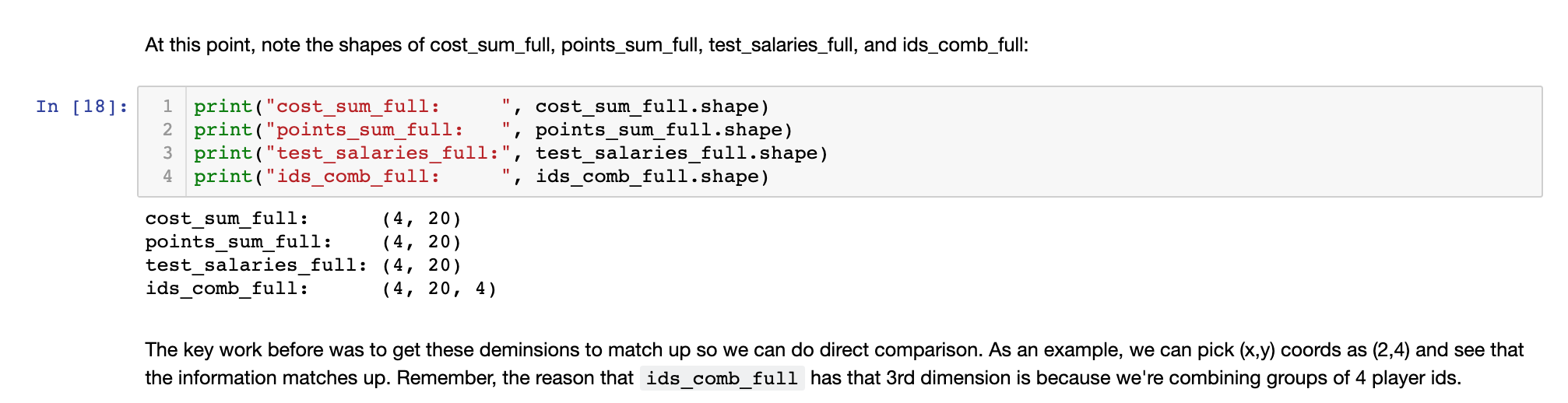
We’re still using for loops to do the math to find the best players whose salaries are less than the cost in the for loop. To solve this, we want to expand those cost, points, and index numpy data structures into another dimension, where there are values for a full 2d matrix of the costs. With those variables, of all the same dimensions, we can do single full_costs <= full_cost_ranges comparison, multiply full_points by that new matrix, find the top indexes by row, and then grab those values to return.

To try to convince you to look at the Jupyter notebook example, here’s a screenshot that shows this point about having the same dimensions.

Here’s a link to the full file on github.

Gif time. This runs damn quick.

In the end, the only thing holding it back is calling numpy.array to cast the list returned by the by the itertools.combinations or .product calls. If this optimization problem was with more players, and I’m talking 1,000s to 100,000s of more players, we’d want to deal with it. But for this project – where people forecast each player’s fantasy points for a particular night and want to know the optimal lineup based on those projections – 0.045 seconds is absolutely quick enough.

Winners on 10/24/2019

This post is about how to optimize, but if you’re here looking for the answer of the best possible lineup of 10/24/2018, here it is:

Stephen Curry PG 9300 61.3
Cameron Payne PG 3700 36.0
Kent Bazemore SG 6700 55.1
Damyean Dotson SG 4100 40.0
Giannis Antetokounmpo SF 11700 78.6
Lance Stephenson SF 3900 47.6
Domantas Sabonis PF 4900 43.0
PJ Tucker PF 4500 32.6
Joel Embiid C 10400 68.8

Combined player points: 463, 430.4 after dropping the lowest score
Combined player salary: $59,200

The Future

Thinking to what’s next, the absolute main thing people would want is to be able to optimize a lineup for that night given given their own projections. I’ve actually made somewhat of an interface locally where we can see the player’s values for a night, their average stats, and make selections to make optimal selections. One of the capabilities of this is for people to select players as keepers – meaning you can select players that you definitely do or do not want to be in your lineup, no matter the result of the optimization. For example, If the Bucks were playing the Celtics that night, pretty sure you’re going to want Khris Middleton on your team. Similarly, when Kawhi is load managing, you’re going to want to make sure he won’t get selected.

Along these lines, if you want to win at DFS NBA, all you need to know is a good estimate of the minutes that people are going to play. This depends on things like load management, and who goes in and out of the rotation. If someone is going to get more minutes tonight than usual, they’re probably worth a pick. To make these picks, we make their projected points their predicted minutes played * average points per 36 which we can calculate. Further, because some of the winnings are top heavy, you can predict points by predicted minutes * std above average points per 36, meaning that you want guys who are playing more minutes but when they get going, they can get really hot.

The final thing to say about this is that I used FanDuel because DraftKings, the other main betting site, has different rules. For them, there’s 1 PG, 1 SG, 1 G, 1 SF, 1 PF, 1 F, 1 C, and 1 Util (meaning any position). This difficulty in this is that we have to make sure nobody who went off on a night isn’t used in three positions. We could quickly test a lineup enforcing 3 PG, 1 SG, 1 SF, 1 PF, 1 F, 1 C, and then test 2 PG, 3 SG, 1 SF, 1 PF, 1 F, 1 C, etc, but that makes us need to check a certain number of position combos.

So, if anyone wants me to do continue with other options, a web UI, and other site capabilities, let me know.

Other thoughts

I always have tons of different thoughts when writing these posts, but I try to do my best to keep all non essential information out of the main body. Let’s be real, people who read this just skim through the words, look at the code to either get inspiration or judge the writer, maybe look at the pictures or stare at the gifs, and that’s it. They don’t want to see random words if they don’t need to, they want technical.

But I like writing about other parts, and some people like reading that too (hi mom), so I throw everything down here in bullet points.

• If someone wants to take that code sample I pasted here and put it in a Jupyter notebook to share with others, please do. Having people run the full code itself takes effort, but following a link, clicking play, and being able to see a dynamic example is much better. You’ll get all the credit too!
• Pandas is great. Like, really great. At first in the normal solution, I had it running at two minutes because I didn’t convert the csv file info into int and floats right away. I looked at the timing logs and saw that was the slowest part of the code, removed them, and it went three times faster. With Pandas, I don’t have to think about conversion. I don’t have to think about calling next(reader) if I don’t want the headings on a csv file. In fact, in the bigger solution I have, I use Pandas to run sql queries in the db where I stored all this data. Like I said, it’s great.
• In the restrict_and_merge function for the fast solution, I was originally using np.tile to expand the dimensions. I realized this was slowing us down the most by looking at the logs. Looking around, I found out that np.tile actually copies the numbers into memory which is a big slowdown. We don’t need that here since all we’re doing is copying the numbers. By using np.broadcast_to, we only tell np that we’re wanting to copy the same numbers to another dimension. I believe np then has a reference to that rather than taking up memory. That cut down the time from ~0.19 seconds to ~0.075, more than 10x quicker. I really, really wanted to include this paragraph in that section itself, but couldn’t convince myself to do that.
• I mentioned this at the top, but I have a bunch of different code that I’ve used to do things like get the data, store the data, and show the data. I used requests and lxml to get the data, postgres to store the data, and flask / vue.js to show and interact with the data. It’s written in python 2 actually, so I’d need to clean it up, upgrade to python 3, and a couple other things before being able to write about it.