Last time, I went through some basics of how naive Bayes algorithm works, and the logic behind it, and implemented the classifier myself, as well as using the NLTK. That’s great and all, and hopefully people reading it got a better understanding of what was going on, and possibly how to play along with classification for their own text documents.
But if you’re looking to train and actually deploy a model, say, a website where people can copy paste reviews from Amazon and see how our classifier performs, you’re going to want to use a library like Scikit-Learn. So with this post, I’ll walk through training a Scikit-Learn model, testing various classifiers and parameters, in order to see how we do, and also at the end, will have an initial, version 1, of a Amazon review classifier that we can use in a production setting.
Some notes before we get going:
- For a lot of the testing, I only use 5 or 10 of the full 26 classes that are in the dataset.
- Keep in mind, that what works here might not be the same for other data sets. We’re specifically looking at Amazon product reviews. For a different set of texts (you’ll also see the word corpus being thrown around), a different classifier, or parameter sets might be used.
- The resulting classifier we come up with is, well, really really basic, and probably what we’d guess would perform the best if we guessed what would be the best at the onset. All the time and effort that goes into checking all the combinations
- I’m going to mention here this good post that popped up when I was looking around for other people who wrote about this. It really nicely outlines going how to classify text with Scikit-learn. To reduce redundancy, something that we all should work towards, I’m going to point you to that article to get up to speed on Scikit-learn and how it can apply to text. In this article, I’m going to start at the end of that article, where we’re working with Scikit-learn pipelines.
As always, you can say hi on twitter, or yell at me there for messing up as well if you want.
How many grams?
First step to think about is how we want to represent the reviews in naive Bayes world, in this case, a bag of words / n-grams. In the other post, I simply used word counts since I wasn’t going into how to make the best model we could have. But besides word counts, we can also bump up the representations to include something called a bigram, which is a two word combos. The idea behind that is that there’s information in two word combos that we aren’t using with just single words. With Scikit-learn, this is very simple to do, and they take care of it for you. Oh, and besides bigrams, we can say we want trigrams, fourgrams, etc. Which we’ll do, to see if that improves performance. Take a look at the wikipedia article for n-grams here.
For example is if a review mentions “coconut oil cream”, as in some sort of face cream (yup, I actually saw this as a mis-classified review), simply using the words and we might get a classification of food since we just see “coconut” “oil” and “cream”. But if we use bigrams as well as the unigrams, we’re also using “coconut oil” and “oil cream” as information. Now this might not get us all the way to a classification of beauty, but it could tip us over the edge.
This is achieved by the ngram_range=(1, 2) parameter in the vectorizer code below. If we passed that into the initializer, then in our bucket, would include all the unigrams (words), as well as bigrams. If we had ngram_range=(2, 2) then we’d only have a bad of bigrams.
For this test here like I said, I’m going to test using uni, bi, tri, and four-gram trained classifiers and see what kind of results we get!
classifier = MultinomialNB()

count_vectorizer = CountVectorizer(min_df=1, stop_words='english'
bigram_vectorizer = CountVectorizer(ngram_range=(1, 2), min_df=1, stop_words='english')
trigram_vectorizer = CountVectorizer(ngram_range=(1, 3), min_df=1, stop_words='english')
fourgram_vectorizer = CountVectorizer(ngram_range=(1, 4), min_df=1, stop_words='english')


unigram_pipeline = Pipeline([
  ('count_vectorizer', unigram_vectorizer),
  ('classifier' , classifier)
])

bigram_pipeline = Pipeline([
  ('count_vectorizer', bigram_vectorizer),
  ('classifier' , classifier)
])

trigram_pipeline = Pipeline([
  ('count_vectorizer', trigram_vectorizer),
  ('classifier' , classifier)
])

fourgram_pipeline = Pipeline([
  ('count_vectorizer', fourgram_vectorizer),
  ('classifier' , classifier)
])

unigram_pipeline.fit(train_data['text'].values, train_data['class'].values)
unigram_predictions = pipeline.predict(test_data['text'].values)
unigram_score = accuracy_score(actual, unigram_predictions)
unigram_cmat = confusion_matrix(actual, unigram_predictions, labels)

print "Unigram"
print unigram_score
print labels
print unigram_cmat

bigram_pipeline.fit(train_data['text'].values, train_data['class'].values)
bigram_predictions = bigram_pipeline.predict(test_data['text'].values)
bigram_score = accuracy_score(actual, bigram_predictions)
bigram_cmat = confusion_matrix(actual, bigram_predictions, labels)

print
print "Bigram"
print bigram_score
print labels
print bigram_cmat

trigram_pipeline.fit(train_data['text'].values, train_data['class'].values)
trigram_predictions = trigram_pipeline.predict(test_data['text'].values)
trigram_score = accuracy_score(actual, trigram_predictions)
trigram_cmat = confusion_matrix(actual, trigram_predictions, labels)

print
print "Trigram"
print trigram_score
print labels
print trigram_cmat

fourgram_pipeline.fit(train_data['text'].values, train_data['class'].values)
fourgram_predictions = fourgram_pipeline.predict(test_data['text'].values)
fourgram_score = accuracy_score(actual, fourgram_predictions)
fourgram_cmat = confusion_matrix(actual, fourgram_predictions, labels)

print
print "Fourgram"
print fourgram_score
print labels
print fourgram_cmat

#output
Unigram
0.90215625
['baby', 'tool', 'home', 'pet', 'food', 'automotive', 'instant_video', 'beauty', 'cds_vinyl', 'clothes']
[[2922 57   92   32   12   20   3    36   9    54  ]
 [ 57  2793 93   19   2    177  4    21   2    60  ]
 [ 176 171  2635 44   72   53   10   25   7    130 ]
 [ 90  57   69   2844 23   35   2    48   3    44  ]
 [ 18  2    82   23   3041 5    2    16   1    8   ]
 [ 39  292  63   19   0    2667 1    39   4    40  ]
 [ 12  4    3    5    4    8    3149 6    19   8   ]
 [ 46  39   43   13   23   20   2    2913 2    96  ]
 [ 3   2    2    1    2    0    25   4    3079 2   ]
 [ 106 58   34   13   3    20   8    30   2    2826]]

Bigram
0.954125
['baby', 'tool', 'home', 'pet', 'food', 'automotive', 'instant_video', 'beauty', 'cds_vinyl', 'clothes']
[[3110 25   39   6    5    8    0    25   10   9   ]
 [ 19  3098 34   6    1    36   2    12   4    16  ]
 [ 48  73   3083 14   31   18   3    16   10   27  ]
 [ 61  44   35   2992 12   8    2    36   2    23  ]
 [ 9   1    39   5    3122 2    1    11   2    6   ]
 [ 13  162  24   2    2    2911 1    27   8    14  ]
 [ 6   2    5    3    1    3    3168 4    23   3   ]
 [ 26  27   28   5    9    1    0    3069 4    28  ]
 [ 0   1    4    0    0    2    4    2    3107 0   ]
 [ 76  65   29   5    2    6    3    37   5    2872]]

Trigram
0.96740625
['baby', 'tool', 'home', 'pet', 'food', 'automotive', 'instant_video', 'beauty', 'cds_vinyl', 'clothes']
[[3141 21   31   4    3    1    0    19   12   5   ]
 [ 15  3143 17   5    0    26   2    7    6    7   ]
 [ 27  71   3143 8    20   9    3    15   9    18  ]
 [ 45  25   22   3064 9    3    2    25   2    18  ]
 [ 8   1    27   5    3148 0    0    5    2    2   ]
 [ 6   125  15   0    1    2984 1    21   6    5   ]
 [ 6   2    3    2    1    3    3171 2    28   0   ]
 [ 19  18   20   4    6    0    0    3111 4    15  ]
 [ 0   0    3    0    0    2    0    2    3113 0   ]
 [ 53  42   23   3    2    5    2    27   4    2939]]

Fourgram
0.97021875
['baby', 'tool', 'home', 'pet', 'food', 'automotive', 'instant_video', 'beauty', 'cds_vinyl', 'clothes']
[[3129 21   13   3    2    0    0    4    0    2   ]
 [ 16  3056 19   6    2    23   0    8    2    7   ]
 [ 36  70   3078 8    17   8    4    6    3    12  ]
 [ 28  40   26   3113 16   1    0    24   2    6   ]
 [ 10  0    18   9    3098 2    0    7    2    0   ]
 [ 16  124  32   2    2    2955 0    12   5    11  ]
 [ 5   0    0    0    3    1    3121 2    49   2   ]
 [ 15  18   12   4    4    2    0    3190 5    8   ]
 [ 0   0    1    0    1    0    3    0    3189 0   ]
 [ 39  34   16   2    0    14   0    17   9    3118]]
And what do you know, having more information about the documents (in the form of more phrases) will get better accuracy!
Now in terms of overfitting, I’m not sure that’s an issue here when using 4 or more grams in the model. The reason we’re getting better performance from those is because these reviews are often of the same form, and use the same phrases. Reviews are sort of a technical document, and if we can get all the technicalities of a review in longer grams, then we can do that. Of course, in production, if we notice we’re not getting the kind of results we expected from training, then we might rethink this, but for now, more grams the better.
For the rest of the testing here however, I’m going to stick with using a bigram vectorizer since training larger-gram vectorizers takes longer, and I don’t want to sit and wait that long when all we’re doing is comparing accuracies. In the end, I can bump to tri or four grams to get final expected results.
Type of Naive Bayes?
Naive Bayes classifiers, specifically the P(word|class) values aren’t just in a single form. In fact, there are three main types of forms for that term — Gaussian, Multinomial, and Bernoulli. You can read about them on Wikipedia here, and how they work in Scikit-Learn land with their docs here.
In this case, Gaussian doesn’t work since our matrices are sparse (and SKL will spit back and angry error if we even try to use that classifier), so we want to evaluate the Multinomial (which is what I used at first) and also Bernoulli.
Below is the code to test each of the classifiers, and we’re running them with the bigram_vectorizer since we’re just looking at relative performance, not overall so we don’t want to waste time on training the tri or four gram models.
mn_classifier = MultinomialNB()
b_classifier = BernoulliNB()

mn_pipeline = Pipeline([
  ('count_vectorizer', bigram_vectorizer),
  ('classifier' , mn_classifier)
])

b_pipeline = Pipeline([
  ('count_vectorizer', bigram_vectorizer),
  ('classifier' , b_classifier)
])

mn_pipeline.fit(train_data['text'].values, train_data['class'].values)
mn_predictions = mn_pipeline.predict(test_data['text'].values)
mn_score = accuracy_score(actual, mn_predictions)
mn_cmat = confusion_matrix(actual, mn_predictions, labels)

print
print "Multinomial"
print mn_score
print labels
print mn_cmat

b_pipeline.fit(train_data['text'].values, train_data['class'].values)
b_predictions = b_pipeline.predict(test_data['text'].values)
b_score = accuracy_score(actual, b_predictions)
b_cmat = confusion_matrix(actual, b_predictions, labels)

print
print "Bernoulli"
print b_score
print labels
print b_cmat

#output
Multinomial
0.9659375
['baby', 'tool', 'home', 'pet', 'food']
[[3124 20   21   7    7   ]
 [ 33  3113 54   13   2   ]
 [ 62  71   3011 17   26  ]
 [ 50  35   57   3025 12  ]
 [ 18  1    29   10   3182]]

Bernoulli
0.91925
['baby', 'tool', 'home', 'pet', 'food']
[[3113 2    5    55   4   ]
 [ 93  2567 85   468  2   ]
 [ 101 18   2764 269  35  ]
 [ 12  16   8    3143 0   ]
 [ 15  0    19   85   3121]]

Multinomial
0.95765625
['baby', 'tool', 'home', 'pet', 'food', 'automotive', 'instant_video', 'beauty', 'cds_vinyl', 'clothes']
[[3101 18   32   1    5    7    2    18   6    15  ]
 [ 23  3055 44   4    4    42   0    11   9    9   ]
 [ 54  63   2984 8    34   14   6    17   6    24  ]
 [ 33  34   33   2999 7    13   0    33   5    12  ]
 [ 13  0    27   7    3156 1    0    12   3    0   ]
 [ 19  119  45   8    3    2959 3    18   2    14  ]
 [ 8   1    3    2    5    2    3135 5    25   1   ]
 [ 29  14   19   4    12   1    0    3120 8    41  ]
 [ 0   0    3    0    3    0    4    0    3150 1   ]
 [ 79  49   34   11   2    12   5    22   10   2986]]

Bernoulli
0.80146875
['baby', 'tool', 'home', 'pet', 'food', 'automotive', 'instant_video', 'beauty', 'cds_vinyl', 'clothes']
[[2571 1    8    13   0    6    0    11   0    595 ]
 [ 5   2038 17   12   0    196  0    3    0    930 ]
 [ 24  12   2093 17   32   24   0    6    0    1002]
 [ 7   6    9    2725 2    19   0    9    0    392 ]
 [ 3   0    6    3    2881 3    0    9    0    314 ]
 [ 2   12   7    7    0    2657 0    1    0    504 ]
 [ 0   0    1    1    0    0    2645 0    0    540 ]
 [ 9   3    0    4    4    1    0    2640 0    587 ]
 [ 1   0    0    1    1    6    187  1    2206 758 ]
 [ 7   6    3    0    0    1    0    2    0    3191]]
It thinks everything is clothes! Look at that last column. You might be tricked into thinking that clothes is the outlier and compared to multinomial, look at the result when we drop the clothes class.
It’s still worse than multinomial.
What if we ran everything through a bernoulli, and use the class it predicts unless it thinks it’s clothes, and then run it as multinomial?
Tfidf
Term frequency inverse document frequency is another way of describing a word document. So rather than turning each document into a dictionary of counts, we turn it into a dictionary of frequencies. You can read up on it more on the Wikipedia article I linked above, and also many other articles on the internet.
In the code below, also note that there also is a TFIDF Vectorizer that we could have used, but having two steps in the pipeline below will get us to the same spot.
pipeline = Pipeline([
  ('count_vectorizer', bigram_vectorizer),
  ('classifier' , classifier)
])

pipeline.fit(train_data['text'].values, train_data['class'].values)
predictions = pipeline.predict(test_data['text'].values)
score = accuracy_score(actual, predictions)
cmat = confusion_matrix(actual, predictions, labels)

print "Bigram"
print score
print labels
print cmat

tfidf_pipeline = Pipeline([
  ('count_vectorizer', bigram_vectorizer),
  ('tfidf_transformer', TfidfTransformer()),
  ('classifier' , classifier)
])

tfidf_pipeline.fit(train_data['text'].values, train_data['class'].values)
tfidf_predictions = tfidf_pipeline.predict(test_data['text'].values)
tfidf_score = accuracy_score(actual, tfidf_predictions)
tfidf_cmat = confusion_matrix(actual, tfidf_predictions, labels)

print
print "Using TFIDF"
print tfidf_score
print labels
print tfidf_cmat

#output
Using TFIDF
0.9493125
['baby', 'tool', 'home', 'pet', 'food', 'automotive', 'instant_video', 'beauty', 'cds_vinyl', 'clothes']
[[3114 23   22   1    8    14   3    16   4    26  ]
 [ 27  3051 49   5    2    89   1    13   1    28  ]
 [ 63  95   2916 17   60   30   4    13   6    52  ]
 [ 41  46   39   2928 15   27   0    48   3    23  ]
 [ 20  1    22   7    3069 6    1    7    0    1   ]
 [ 16  116  42   3    1    2880 3    32   5    32  ]
 [ 7   2    2    2    8    2    3104 8    25   5   ]
 [ 23  31   21   5    19   4    2    3124 6    40  ]
 [ 0   0    1    0    2    1    6    2    3188 6   ]
 [ 57  27   17   2    4    19   5    27   5    3004]]

Not Using TFIDF
0.95303125
['baby', 'tool', 'home', 'pet', 'food', 'automotive', 'instant_video', 'beauty', 'cds_vinyl', 'clothes']
[[3124 22   23   3    3    11   3    17   3    22  ]
 [ 21  3099 49   2    2    57   1    10   3    22  ]
 [ 56  91   2993 3    32   25   2    15   6    33  ]
 [ 38  49   31   2962 8    19   0    44   2    17  ]
 [ 17  1    30   8    3061 4    1    11   0    1   ]
 [ 20  125  45   6    5    2879 3    25   3    19  ]
 [ 6   2    6    0    9    1    3101 9    29   2   ]
 [ 21  29   27   6    18   6    2    3129 3    34  ]
 [ 2   0    2    0    2    1    5    2    3188 4   ]
 [ 79  31   29   10   0    14   5    27   11   2961]]
Using the TFIDF transform, we get hit with a 0.4% drop in accuracy. Not much but I’m not going to use it if we’re not getting better results. Really, it seems, TFIDF is a good heuristic for smaller data sets where you’re not accounting for stopwords for example. Here we remove stopwords, and have a large data set, so we don’t really need the TFIDF mechanism.
Effect of amount of training examples
So far, I’ve been using 80,000 total data points for the original 5 classes, 64,000 used for training, and 16,000 used for testing, following the “train with 4/5, test with 1/5” mantra.
I figure now would be a good time to see the effect on accuracy score using variable amounts of data. Common sense would say that the more samples you use, the better the accuracy. Let’s see if that’s the case.
Total Samples: 10000
0.891
['baby', 'tool', 'home', 'pet', 'food']
[[414 4   8   8   4  ]
 [ 7  324 13  5   3  ]
 [ 34 46  289 14  16 ]
 [ 24 14  1   352 5  ]
 [ 2  0   5   5   403]]

Total Samples: 20000
0.9015
['baby', 'tool', 'home', 'pet', 'food']
[[746 19  15  7   2  ]
 [ 28 732 33  7   3  ]
 [ 54 58  640 8   20 ]
 [ 33 32  29  713 8  ]
 [ 9  2   23  4   775]]

Total Samples: 30000
0.915333333333
['baby', 'tool', 'home', 'pet', 'food']
[[1122 21   26   16   5   ]
 [ 23  1125 47   12   4   ]
 [ 78  67   1026 17   31  ]
 [ 30  43   36   1064 18  ]
 [ 4   1    20   9    1155]]

Total Samples: 40000
0.92375
['baby', 'tool', 'home', 'pet', 'food']
[[1566 32   42   8    3   ]
 [ 28  1523 53   6    6   ]
 [ 88  81   1352 25   59  ]
 [ 53  34   32   1441 9   ]
 [ 8   3    26   14   1508]]

Total Samples: 50000
0.9351
['baby', 'tool', 'home', 'pet', 'food']
[[1912 29   38   14   4   ]
 [ 27  1905 45   16   5   ]
 [ 93  104  1727 16   39  ]
 [ 57  44   49   1830 17  ]
 [ 9   3    27   13   1977]]

Total Samples: 60000
0.948
['baby', 'tool', 'home', 'pet', 'food']
[[2352 28   39   9    6   ]
 [ 30  2339 53   10   2   ]
 [ 85  82   2166 19   54  ]
 [ 38  49   43   2183 13  ]
 [ 13  4    31   16   2336]]

Total Samples: 70000
0.950357142857
['baby', 'tool', 'home', 'pet', 'food']
[[2654 33   34   5    6   ]
 [ 44  2659 52   6    3   ]
 [ 99  96   2534 17   54  ]
 [ 52  75   44   2624 8   ]
 [ 17  1    38   11   2834]]

Total Samples: 80000
0.9574375
['baby', 'tool', 'home', 'pet', 'food']
[[3010 33   32   2    5   ]
 [ 40  3072 51   6    2   ]
 [ 85  89   2944 26   35  ]
 [ 73  74   51   3080 15  ]
 [ 13  3    36   10   3213]]
Would you look at that, more data means more accuracy. Not much interesting here, but a good test to make sure things are looking right. If I had gotten worse accuracy with the increasing data, that’d be a sign there was a problem that I should be looking into.
Priors
Up until now, it’s been mostly plug and chug — there are a few different options for how to describe the documents, and a few different options for classifiers. All we have to do is try each and see which ones perform the best and then go with that.
Going back to Bayes’ Rule, remember that besides the terms for P(word|class), there’s also a leading term, P(class) which we’ve been basically ignoring up until now. That term accounts for the probability that we see a document of that class in the first place, and is basically the foundation of Bayes’ Rule. If we don’t expect to see a document of a certain class, like if we see reviews for tools 5 times more than reviews for baby products, then in order to classify a review as baby, we need to be really certain based on the words in the review that we’re hearing about babies.
In our case, what priors do we want, if any? In our use case here, just a simple test of the system where people copy and paste reviews to see if we guess correctly for fun, we pretty much have no idea what they’re going to input. So for now, the classifier is going to start with an even distribution for the prior probabilities, meaning that we think there’s an even chance a person will upload a review from all 26 of the classes. Perhaps later versions of the classifier can use the information for which types of reviews we actually see from people, but for now, no guessing.
The Big One
At this point, we’ve done pretty well here in figuring out which types of vectorizers and classifier type we want to use to get the best results here, so now is a good time to go all out — all 26 classes, with the four-gram vectorizer.
0.932907608696
['baby', 'tool', 'home', 'pet', 'food', 'automotive', 'instant_video', 'beauty', 'cds_vinyl', 'clothes', 'digital_music', 'cell_phones', 'electronics', 'kindle', 'movies_tv', 'instruments', 'office', 'patio', 'health', 'sports', 'toys', 'video_games', 'books']
[[3052 10   7    0    2    3    0    3    2    0    0    3    5    0    0    1    29   32   9    0    40   6    0   ]
 [ 4   3025 14   0    0    11   0    7    0    4    0    9    18   0    2    3    59   108  0    13   4    20   0   ]
 [ 25  31   2940 2    7    3    0    1    0    8    4    0    3    0    0    2    45   138  8    0    3    11   2   ]
 [ 14  5    4    2886 8    6    0    24   1    6    0    2    6    0    0    1    9    121  24   0    15   8    0   ]
 [ 3   0    18   0    3134 0    0    6    2    0    1    0    0    0    1    2    4    14   20   0    5    2    6   ]
 [ 6   51   2    0    0    2868 0    2    0    1    3    3    33   0    0    2    22   92   2    9    2    19   0   ]
 [ 0   0    0    0    4    0    2735 0    2    2    20   0    1    7    276  0    1    0    0    0    25   48   44  ]
 [ 5   2    6    2    8    0    0    3112 0    7    3    0    3    0    1    2    21   21   19   0    7    18   0   ]
 [ 0   0    0    0    0    0    0    0    2831 0    403  0    0    0    14   0    0    3    0    0    1    3    0   ]
 [ 17  7    7    2    0    3    0    10   0    2936 4    4    16   0    4    1    37   26   3    20   45   36   0   ]
 [ 0   1    0    0    0    0    0    2    77   0    3121 0    2    0    0    0    0    0    0    0    0    0    0   ]
 [ 4   2    3    0    1    6    0    0    0    3    7    3013 82   0    2    2    37   15   2    0    7    18   0   ]
 [ 2   6    0    0    0    5    0    0    3    5    3    58   3008 0    2    8    47   23   2    4    6    40   0   ]
 [ 0   0    0    0    9    0    0    0    0    0    2    5    6    2755 14   0    2    1    2    0    0    7    349 ]
 [ 0   0    2    0    1    0    33   3    20   2    8    0    8    4    3136 0    1    0    0    0    0    20   8   ]
 [ 0   19   0    3    0    9    0    5    5    2    0    2    22   0    0    3054 21   24   2    0    3    21   0   ]
 [ 4   3    0    0    0    2    0    0    0    0    0    2    6    0    0    2    3133 0    0    0    0    4    2   ]
 [ 2   6    5    0    0    10   0    0    0    0    0    2    2    0    0    0    5    3182 2    2    0    3    0   ]
 [ 18  9    8    6    53   2    0    72   2    11   6    2    17   0    0    2    34   62   2793 4    3    32   0   ]
 [ 10  37   15   4    6    9    0    8    0    33   2    8    19   0    0    6    56   118  4    2853 10   48   3   ]
 [ 23  2    4    2    0    1    0    2    1    2    2    2    4    0    8    2    16   24   0    4    2963 103  2   ]
 [ 0   0    0    0    0    3    2    0    2    0    2    11   15   0    0    3    12   4    0    0    13   3118 3   ]
 [ 1   0    2    0    4    0    0    0    6    0    4    0    0    127  24   0    2    2    0    0    8    20   3014]]
Why Are We Still Getting Mistakes?
93% is pretty damn good. But what about that 7%? Why are we still getting errors? And is there anyway to fix that within the Naive Bayes constraints?
Length of reviews
More data means better classification rates for sure. So does that hold with length of reviews? Check out the histogram for word counts on the reviews here. I expected an exponential decay type of distribution, and that’s what we got.
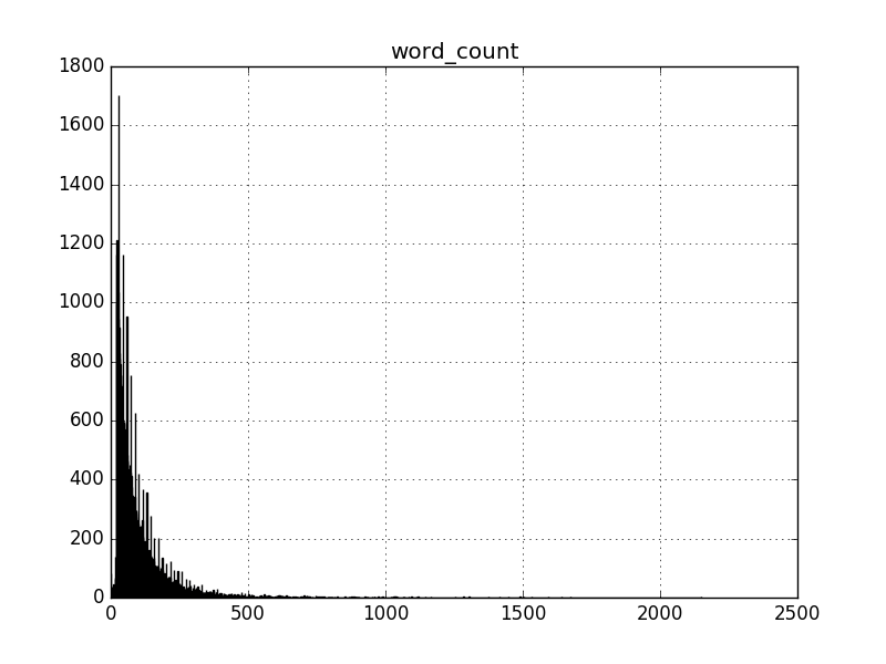
Looks nice, except for that beginning part.
Zooming in here, looking for the word count where we bump up, and it looks like 20 words is some sort of cutoff.

Who writes 20 word reviews anyway?
Running the classifier with ranges of word lengths, we get the following accuracy scores with bigram vectorizer and 10 classes. Again, with more data (words in a review, in this case), we get higher accuracy.
20 Word Max
0.792656587473

Between 25 and 50 Words
0.937370020797

Between 50 and 100 Words
0.964392717216

100 Word Min
0.981591937474
Clearly shorter reviews are tougher to classify. One word in there that is usually associated with a different class and we’d be screwed. Not much you can do here in this case.
“My cats love it too! Exactly what I needed for my babies. Bright light, long battery life, compact, easy to use- It’s a laser- what else is there to say?”
Actual class: pet, Guessed class: tool
You can absolutely see here how the algorithm gets this one wrong. Lights, battery, compact, lasers, all words that more often describe tools than pet products. But that doesn’t mean the result is correct.
Another example:
Very gentle on my dog. Smells nice and leaves her coat nice and soft. Would buy again
Actual: pet, Guessed: beauty
Though the review mentions “dog”, that one word alone apparently wasn’t enough to overcome the words “nice” and “soft”.
Similar Classes
Movies and TV and Instant Video. Tools and Automotive. Books and Kindle. Digital Music and Cds and Vinyl. These classes are so close together that you could reasonably argue that those should be just one class, and you can see with the confusion matrices that these classes get confused with each other way more often than normal. It’s also worth noting that even though they’re basically the same thing, the classifier gets the correct class still way more often than not. Impressive there.
Generic Reviews
Sometimes, like the reviews above, the algorithm messes up and guesses the incorrect class even though us humans know the real answer. But sometimes, humans would get the classification incorrect too.
The battery dies in a matter of months. Shame on you, Black and Decker!!!!!
Actual: home, Guessed: tool
Wouldn’t have guessed home here either.
I bought this as a treat for my cat. I mix it into his wet food to help him eat it. He says it’s delicious.
Actual: food, Guessed: pet
Shoutout to a talking cat!
Research for Version 2
With all that in mind, I’m going to say that for our case here, a simple web interface that can be used to classify text that people input, we have a pretty good first version of the classifier. But as all good tutorials should do, I’m going to mention some possible ways to improve classification accuracy for a second version.
Knowing when you don’t know
Naive Bayes calculates the probability for each class, and Scikit-learn pipeline classification actually has functionality for outputting the relative probabilities for each class. There are some questions here about
For example, if the classifier thinks there’s more than a 50% chance the review belongs to a class, what percentage of those guesses are correct?
Might there be some better way to get.
Knowing error rates for the individual classes
Are there some classes that we get incorrect more often than others? Maybe there’s a way to know that beforehand, and adjust the
Ensembles
When you hear ‘ensemble’ in terms of machine learning algorithms, all that means is using combining classifiers, or using different classifiers in different cases.
If you know of any more ways to improve the model, reach out on twitter, or the contact page on the site, and I’d love to hear from you. Next time, productionizing the model so we can use it in a web app.
